How DoorDash Built an Ensemble Learning Model for Time Series Forecasting

In real-world forecasting applications, it is a challenge to balance accuracy and speed. We can achieve high accuracy by running numerous models and configuration combinations and we gain speed through running fast, computationally inexpensive models. We explore a number of models and configuration combinations at DoorDash to forecast demand on our platform. However, the challenge is to build a forecast model that is highly accurate while also running fast and cheap. To address this  accuracy vs. speed and cost tradeoff,  our forecasting team built a new model called ELITE for Ensemble Learning for Improved Time-series Estimation. The new model uses ensemble models for forecasting instead of optimizing one individual model — allowing computationally efficient models to combine in a way that increases overall accuracy.

Here we discuss how we developed this ensemble model approach to:

• maintain accuracy while significantly reducing runtime, making it feasible to generate forecasts on targets with high dimensionality.
• generate huge computation cost savings through:
  • applying a computationally efficient training framework.
  • optimizing on the infrastructure settings to accommodate the training process on Ray cluster, which was also leveraged by OpenAI for GPT training.
• reduce maintenance effort by creating a highly automated framework to swap in any models.

Limits on forecasting with an individual model pipeline

In recent years, forecasting models have advanced from traditional time series frameworks to increasingly complex deep learning architectures in order to capture the volatile dynamics of real-world scenarios. However, subjectively picking a single model to make accurate forecasts for every target is unrealistic. Therefore, in many industrial practices, a forecasting toolbox applies a selection framework to explore a wide range of models and configurations, carefully evaluating each model's performance on each target before generating final forecasts from the best performer. The configuration space includes not only model parameters, but also options for processing data such as data cleaning, transforming, and outlier handling as well as causal factors, including holidays, weather, or promotions. At DoorDash, we’ve built a forecast factory to enable these functionalities.

But this type of forecasting pipeline is limited by its computational burden. Beyond the complexity of training increasingly complicated model structures, configuration combinations grow exponentially when we add an additional option to each entry. For example, suppose we have 10 configs and each config has two options, meaning we have 2¹⁰ combinations. When we add an additional option to a single config, the config combinations increase by 2⁹. As a result, we must search exhaustively, for instance via a grid search, over thousands of config combinations for each forecasting target, consuming hours of execution time and hundreds of dollars in computational cost per run. Moreover, a rolling window cross-validation process must be applied to evaluate each model’s forecasting performance. Although this grid search method maintains high accuracy for a wide range of forecasting targets, it also significantly increases both runtime and computation costs as we support more use cases. 

At DoorDash, forecasts are generated for highly granular targets, which makes running forecasting models more computationally expensive or even prohibitive. For example, we have tens of thousands of targets when we make forecasts on delivery time in switchback-level experiments to create covariates for variance reduction. But computational limits could block these  use cases because of unacceptably long running times or high cluster costs. These limits prompted development of a new forecasting framework that could reduce the computation budget while maintaining high accuracy.

While ideally we would leverage a single forecasting model, such models come with their own limitations that make them hard to use by themselves, including: 

• Unrealistic assumptions: The model structure may have been simplified with assumptions that are not easily satisfied. For example, a single seasonality assumption would not be able to meet reality’s complex multiple seasonality patterns —inherent to a seven-day week or 52 weeks in a year.
• Biased strength: Some models may only have advantages in making forecasts at particular stages along the forecasting horizon. For example, a model with extreme weather processors may outperform when the weather shifts suddenly, but underperform when during normal trend and seasonality patterns. These limits become particularly critical in long-term forecasting as the deviant trends and patterns accumulate along the forecasting horizon.
• General instability: Forecasts from a single model are relatively less stable. They may produce sharply increasing/decreasing patterns or extreme values that prove unreliable from a business perspective.

Moving to an ensemble model to get the best of both worlds

To solve this real-world forecasting challenge, we proposed a temporal stacking ensemble learning approach. The idea is this: Instead of relying on a single model, we would stack another layer on top of the base candidate models (learners), creating an ensemble of their outputs to obtain the final forecasts. As shown in Figure 1 below, the design of this framework applies two layers of parallelization to maximize the computational efficiency and allow arbitrary choice of the base layer and the ensemble layer models.  

This implementation approach offered several benefits in the form of higher accuracy, better efficiency and cost, better extensibility, and smaller operating risks, as detailed below.

Improved accuracy

The stacking ensemble model achieves less bias than any single base model and could even outperform Bayesian model averaging. Intuitively, each base learner has strengths in capturing the temporal pattern at discrete periods along the forecasting horizon. The stacking ensemble model combines their forecasts to capture benefits from each base, which results in more accurate forecasts. For example, our team ran experiments on weekly order volume across several thousand DoorDash submarkets; results showed that ELITE was about 10% more accurate than the best single model. 

In fact, our proposed ensemble model decently addresses the performance limitations of forecasting with a single model in each aspect discussed in the previous section. Making forecasts from multiple models weakens the imposed model structure assumptions from each single model; using an ensemble model extracts the strengths, resulting in the combined forecasts taking full advantage of the strong performers at different forecasting stages. Furthermore, with diverse base models, the ensemble model produces more stable forecast values.

Improved efficiency and lower costs

The proposed temporal ensemble framework eliminates the need for heavy rolling window cross-validation, which reduces both running time and computational costs. An experiment on our most complex forecasts reduced the model training time from hours to minutes and lowered compute costs more than 80%. The ensemble framework also unblocks complex objectives, including our highest granularity forecasting jobs. For example, at DoorDash we use forecasts to support experimentation variance reduction for delivery time at the highly granular switchback level while the grid search framework failed to finish within an acceptable amount of time. 

More modularization and extensibility

As we built a standardized module wrapper in the ensemble modeling framework, our implementation improved flexibility by supporting any user-defined model. Additionally, the model accepted external features, which means it can support machine learning and deep learning models that require them. This framework also provides valuable information for investigating base models by tracking how their forecasts contribute to the ensemble forecasts. Such base model diagnostic analysis helps model developers better understand how each base model captures a target’s changing patterns.

Lower system maintenance and risk

ELITE doesn’t select the best model performer from base models, which avoids the extra effort of training each model repeatedly on a sequence of run dates along the historical timeline. This simplifies what otherwise can be a complicated model validation process, reducing maintenance  efforts. Because the construction of ELITE only relies on the estimated effect from each base learner, we sharply reduce the number of times we need to train base models. This reduced burden also improves system stability in distributed jobs, reducing the risk of hitting computational limits. 

Building ELITE

We summarize below the main components involved in building our ensemble solution from the perspective of both model workflow and architecture. 

Designing ELITE’s workflow

As shown in Figure 1, our ensemble model solution applies a two-layer — base and ensemble —  architecture. The idea is to use forecasts from the base layer to create a set of features to fit the model in the ensemble layer. In particular, the base model forecast features could be combined with other external features such as causal factors or any other correlated variables to feed into the top-layer machine learning model. In this way, variations in the forecasting target could be fully captured by its temporal expectations under various time series model assumptions as reflected in  base model forecasts as well as by factors from other sources through external features.

We created the ensemble forecaster through the following steps, which we detail below:

1. Choosing a set of base learners 
2. Applying a stacking temporal k-fold cross-validation strategy to generate forecasts from base learners to fit the top-layer ensemble forecaster
3. Choosing and fitting the top-layer model and making the final forecasts

How we chose base learners

The forecasting capability of ELITE depends on its potential for adopting different base learners. The centralized forecasting platform at DoorDash supports a wide range of candidate models and configurations. 

In addition to integrating forecasting models from existing packages such as statsmodels, prophet, and lightgbm, we customize models by introducing many configurations. These configurations include both the underlying model structures including internal configurations such as additive or multiplicative trends, seasonality, or error assumptions), as well as time series processing options for external configurations, including how to handle missing values and outliers and whether/how to adjust for impacts from holidays, weather, or promotions. These flexible options provide a great source of models for ELITE.

Ensemble model forecast accuracy can be improved by promoting diversity among the base models. To support this, we developed a standardized model wrapper layer to further incorporate new models, an approach we’ll discuss in more detail below. We plan future research into other options for improving accuracy, such as penalizing base model complexity.

Stacking temporal k-fold cross validation

It is crucial to estimate the effect of each base model as we create the ensemble forecaster. As shown in Figure 2, we estimate the base model effect through a stacking temporal k-fold cross-validation framework which fits a model on observations versus the stacked forecasts for each validation block. In this temporal cross validation framework, the temporal order of the data will be preserved. 

The stacking temporal k-fold cross-validation procedure follows these steps:

1. Partition the dataset into n segments
2. In each segment, create k-folds and

• Fit each base learner with data from the training periods
• Collect both forecasts and actuals for each base learner from the testing periods 

3. Stack the forecasts and actuals for each base learner generated in step 2 and fit them in the ensemble layer to obtain the effect, or weight, for each base learner

Choosing an ensemble learner

When fitting the ensemble model layer, the selection of models should be based on the number of independent variables — base models — and the data sample size, or stacked observations. A large number of base learners and sufficient data would favor more complex model structures. It is important to choose models that are not sensitive to correlated samples, especially for temporal data. Our architecture allows for flexibility in selecting models with different levels of complexity, ranging from linear regression to neural networks.

Implementing ELITE architecture

To implement this ensemble design, we integrated the framework with our Forecast Factory code base. We decomposed the training process of ELITE into key components, such as training base learners, stacking temporal k-fold cross validation, and training the ensemble layer, and created an ensemble model class that incorporates each of their implementations. Then we created a generic runner class for running the ensemble forecasting workflow. This runner can easily be inherited and adapted to any of our existing forecasting jobs. With this implementation, we can apply a nested parallelization framework; the design also allows us the flexibility to make model choices in the base and ensemble layers within our architecture. In the next section, we discuss how this design offers significant advantages in efficiency and generalizability, particularly  when dealing with high-granularity forecasting targets.

Nested parallelization on the Ray cluster

To maximize forecasting job efficiency, we implemented a nested parallelization framework in our ensemble modeling design to simultaneously generate forecasts for a large number of targets. As shown in Figure 3, our nested parallelization framework involves parallel training of each target in the outer layer and parallel training of each base learner in the inner layer. Without this framework, training millions of individual forecasting models sequentially would be time-consuming and computationally prohibitive.

To provide a stable distributing environment and fully utilize the benefits of our nested parallelization across nodes on both layers, we adopted Ray, a new distributed training framework that makes scaling easier. With KubeRay, we launched the Ray clusters on our in-house Kubernetes infrastructure and maximized our ensemble model’s efficiency, significantly reducing both execution time and computation cost.

Flexible model choices with generic model wrappers

Our architecture also provides the benefit of generalizability derived from the generic design of our base model and ensemble model wrappers. Our standardized implementation framework enables us not only to integrate models from existing machine learning, deep learning, or forecasting packages, but also lets users create customized model classes based on their specific needs. 

The DoorDash use case

Here we will present two DoorDash use cases to demonstrate our ensemble model’s performance. 

The first case involves weekly order volume forecasts to enable financial and operations planning for several thousand submarkets. We explore thousands of different model and configuration combinations for each submarket; each combination corresponds to one base learner. As shown in Table 1, we observed significant efficiency and accuracy improvement with ELITE as compared to grid search. We achieved 78% and 95% reduction in execution time and computation cost respectively as well as 12% MAPE accuracy improvement. 

	% improvement of ELITE over grid search
Cluster Type	Execution Time	Cluster Cost	Accuracy (MAPE)
Spark	83%	96%	12%
Ray*	78%	95%

*Note that the improvement percentages shown in Table 1 compare ELITE to grid search on the same cluster type. However, running ELITE on Ray reduces the execution time and cost compared to running ELITE on Spark, as shown in Table 2.  

The second use case involves our delivery time forecast as an example to support experimentation variance reduction. This forecast is made at the switchback level, which is our experimentation randomization unit. With the number of five-digit switchback units at DoorDash, grid search could not provide a feasible solution within reasonable computational budget and time constraints. However, ELITE generated these highly granular forecasts within an hour and 20 minutes with 10% variance reduction improvement over using a multiple lagged historical time series, for example, CUPED. 

For such highly granular forecasts, we would like to highlight the efficiency-improving power generated by combining our ensemble algorithm with the Ray infrastructure. The minimum computational burden achieved by the ensemble algorithm allowed  us to execute the model on small and inexpensive  Ray clusters. As a result, in addition to unblocking the forecasting job from grid search, we also reduced our execution time and computation cost by switching to Ray from Spark clusters, as shown in Table 2.     

	Execution Time vs. Spark	Cluster Cost vs. Spark
Improvement by Ray	50%	93%

Drawbacks to ELITE

Despite all of the advantages, there are a few drawbacks to using ensemble models that we plan to address as we develop further improvements in accuracy. Although ELITE improves forecasting accuracy over a single model in most common scenarios, its ability to handle extreme cases is inferior to a single highly specialized model. The deficiency comes from the single model’s ability to capture a particular extreme pattern; when its forecasts are combined with others that are less representative of that pattern, accuracy drops. On the other hand, as shown in Figure 4, highly diverse base learner combinations provide high accuracy for most common scenarios,  comprehensively covering the variation from as many directions as possible.

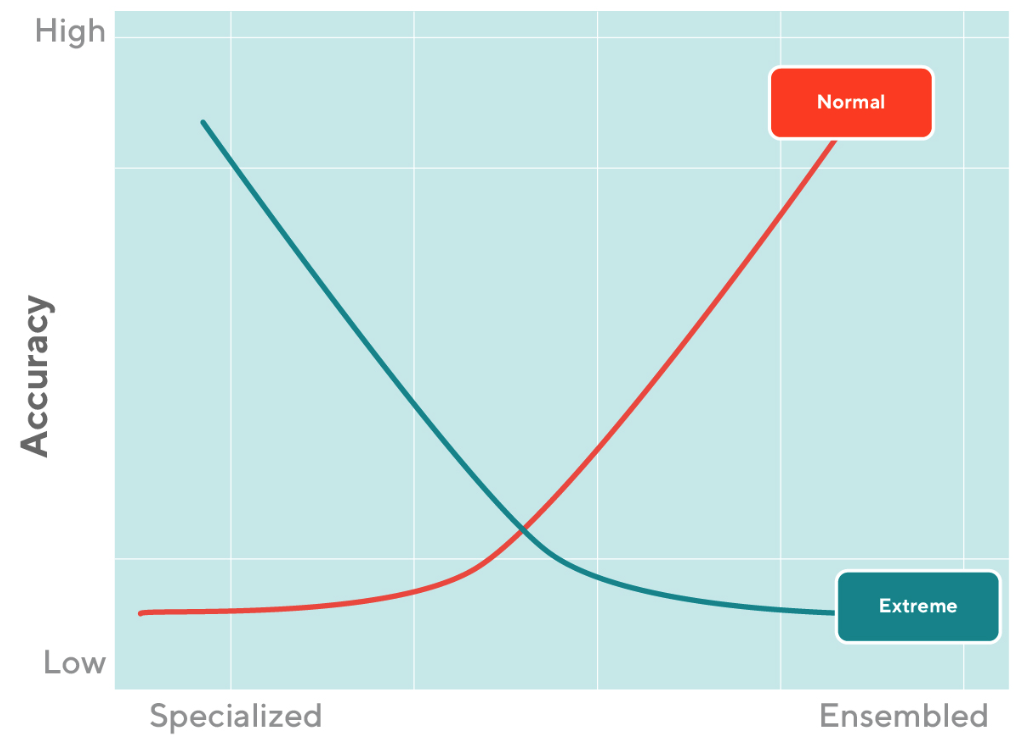
For an extreme scenario, accuracy increases as the model becomes more specialized (along the inverse direction of x-axis) and decreases as the model becomes more ensembled (along the x-axis). On the other hand, for a common scenario, the accuracy increases as the model becomes more ensembled (along the x-axis) and decreases as the model becomes more specialized (along the inverse direction of the x-axis).

To counter these conflicted preferences on specialized and ensemble models when dealing with different data patterns, we plan to focus on exploring more intelligent ways to create an ensemble of base learners to find a balance in overall accuracy tradeoffs. We then plan to optimize our use of an individual learner's ability to assess extreme situations while continuing to maintain model diversity to guarantee accuracy and robustness under most common scenarios.

Learning from improving execution efficiency

In closing, we would like to share some insights that we gained while building our ensemble model solution. 

The importance of backend choice and setup

Backend infrastructure plays a crucial role in building efficient and reliable machine learning solutions. As we discovered during our initial execution of the nested parallelization framework with the Spark backend on Spark clusters, we experienced difficulties in debugging with non-informative logs on the driver node. 

Good implementation practices

Constant refactoring can lead to significant efficiency gains and is an ideal programming practice, especially when developing code that includes complicated parallelization structures. At the beginning of our parallel implementation, for example, we directly passed the whole class object (self) to many parallelized methods, which resulted in unacceptable slowdowns in data distributions and executions. However, after refactoring to minimize the data and objects passing through these parallelized methods, we achieved more than six-fold efficiency improvements.

Conclusion

The proposed ensemble framework is applicable not only to the specific forecasting problem we addressed but also to any forecasting system that requires a heavy model selection process. It also serves as a powerful machine learning system where time series forecasting features such as weather could be included in addition to stacked model predictions. By establishing ensemble connections between base models, the proposed framework offers the flexibility to support both machine learning and forecasting use cases, resulting in higher accuracy and efficiency benefits — without the need for a complex deep learning pipeline. 

Acknowledgements

We truly appreciate all the help and support from the DSML forecasting and MLP forecasting teams —  Swaroop Chitlur, Ryan Schork, Chad Akkoyun, Hien Luu and Cyrus Safaie who made  this collaborative project possible and successful. Many thanks to Joe Harkman, Robert Kaspar and Stas Sajin, who shared incredibly valuable insights and suggestions in the design review of this work. Our appreciation also goes to the experimentation platform team partners Bhawana Goel, Caixia Huang, Yixin Tang and Stas Sajin for their efforts and collaboration discussing and onboarding the use cases. Finally, many thanks to the Eng Enablement team for continuous support, review, and editing on this article.