Introduction
In this second blog article, we’ll walk through the steps for downloading a 30-year time series of daily precipitation rasters, then processing this raster data into a tabular dataset where each row represents a location in a 4km by 4km grid of the US, along with four different precipitation variables relating to amount, frequency, and variability. These variables are calculated for each season in the 30-year period, totaling 120 seasons. All the following steps are done in R.
The precipitation data
The raw data used in this analysis comes from the Parameter-elevation Regressions on Independent Slopes Model (PRISM) dataset, provided by the PRISM Climate Group at Oregon State University. The dataset contains a 30-year (1981-2010) time series of daily precipitation (mm) gridded raster data at 4km by 4km spatial resolution. Doing some quick math, this is 30 years x 365 days = ~11,000 daily rasters x ~ 481,631 pixels per raster = ~5.3 billion pixels to be processed!
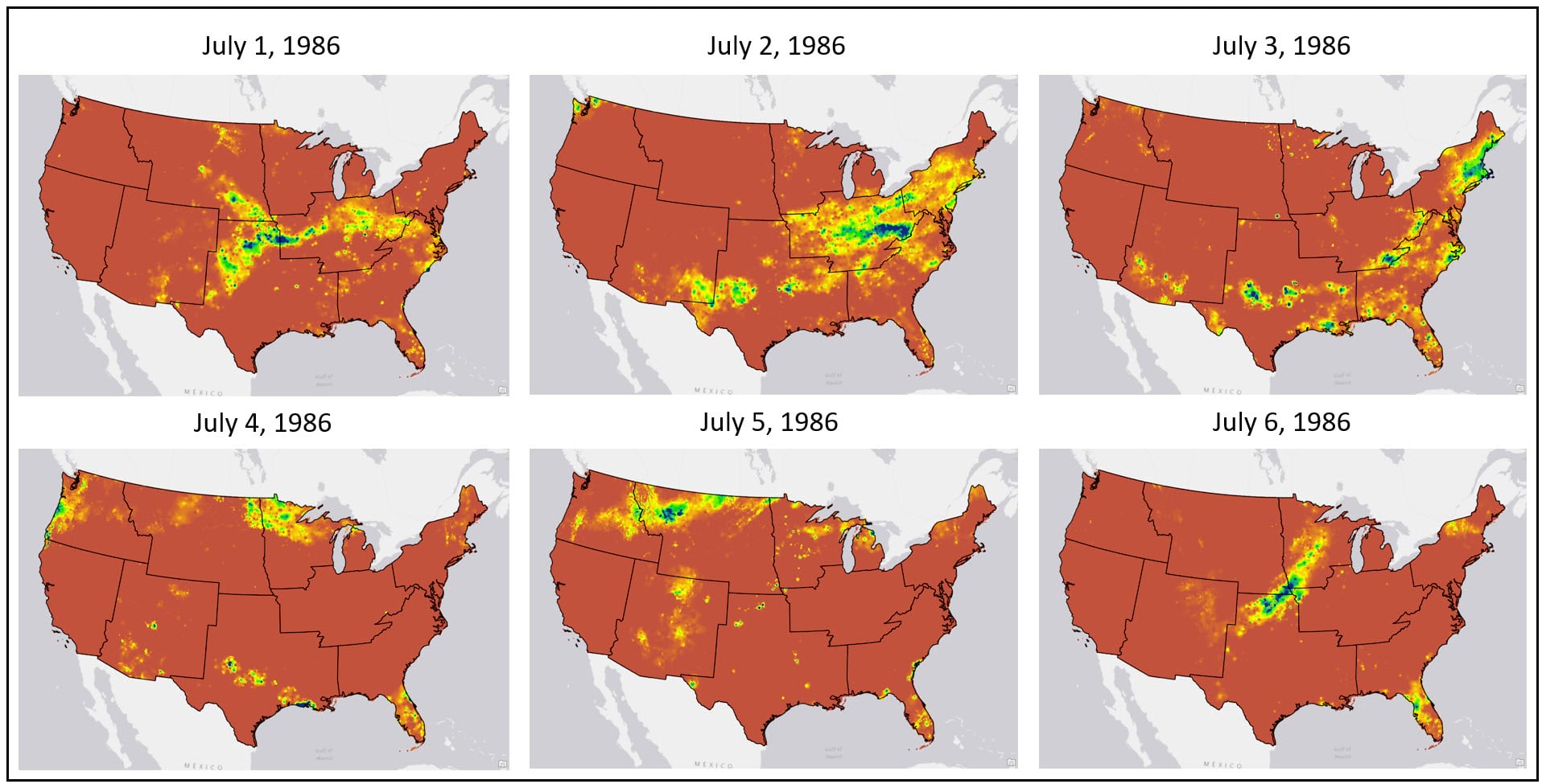
Because we are using seasonal variation in precipitation over time as our proxy for delineating US climate regions, we need to determine 1) what are our metrics for “seasonal variation” and 2) how do we calculate these metrics from a 30-year time series of ~11,000 daily precipitation rasters?
Seasonal variation in precipitation is represented by 4 different precipitation measures.
- Total precipitation – total millimeters (mm) of precipitation within a season
- Frequency of precipitation – total number of precipitation days within a season
- Gini Coefficient – quantifies the variability of precipitation events within a season
- Close to 0 = less variability in precipitation across a season, with each precipitation event having similar amounts, much like a uniform distribution
- Close to 1 = more variability in precipitation across a season, where there is large variation in the amount of precipitation received from event to event
- Lorenz Asymmetry Coefficient – quantifies the kind of precipitation events (heavy or light) within a season by measuring the degree of inequity in the temporal distribution of precipitation
- Less than 1 = variability in the precipitation across a season caused by many, small precipitation events
- Greater than 1 = variability in the precipitation across a season caused by a few large precipitation events
For each location, we need to average each of these four precipitation measures for each season, for every year from 1981-2010. This will result in a time series of 120 seasonal averages (4 seasons per year x 30 years) of each variable, which we will then average over the entire time period. Thus, our final dataset will contain the 30-year average of the four precipitation variables for each season (16 total precipitation variables).
That sounds really complicated. Let’s walk through the process step-by-step and see how we did it!
R packages
In pretty much any R script, it’s very likely that the first few lines of code are for loading the R packages that you need for your task. In this case, I use the library function to load the handful of packages I need.
- {prism} – API for downloading PRISM climate data from Oregon State University
- {raster} – working with raster data
- {reshape2} – reshaping, restructuring, and aggregating tabular data
- {ineq} – measuring inequality in data distributions
- {reldist} – methods for comparing data distributions
- {lubridate} – working with dates
- {dplyr} – working with and manipulating data frames
- {tidyr} – creating “tidy” data (cleaning, wrangling, manipulating data frames)
Accessing the data
Fortunately, the {prism} package can be used to programmatically access PRISM data. Within this package, there are a series of functions that allow you to choose which variable and temporal scale you want to download. In my case, I was interested in daily precipitation data, so I used the get_prism_dailys function.

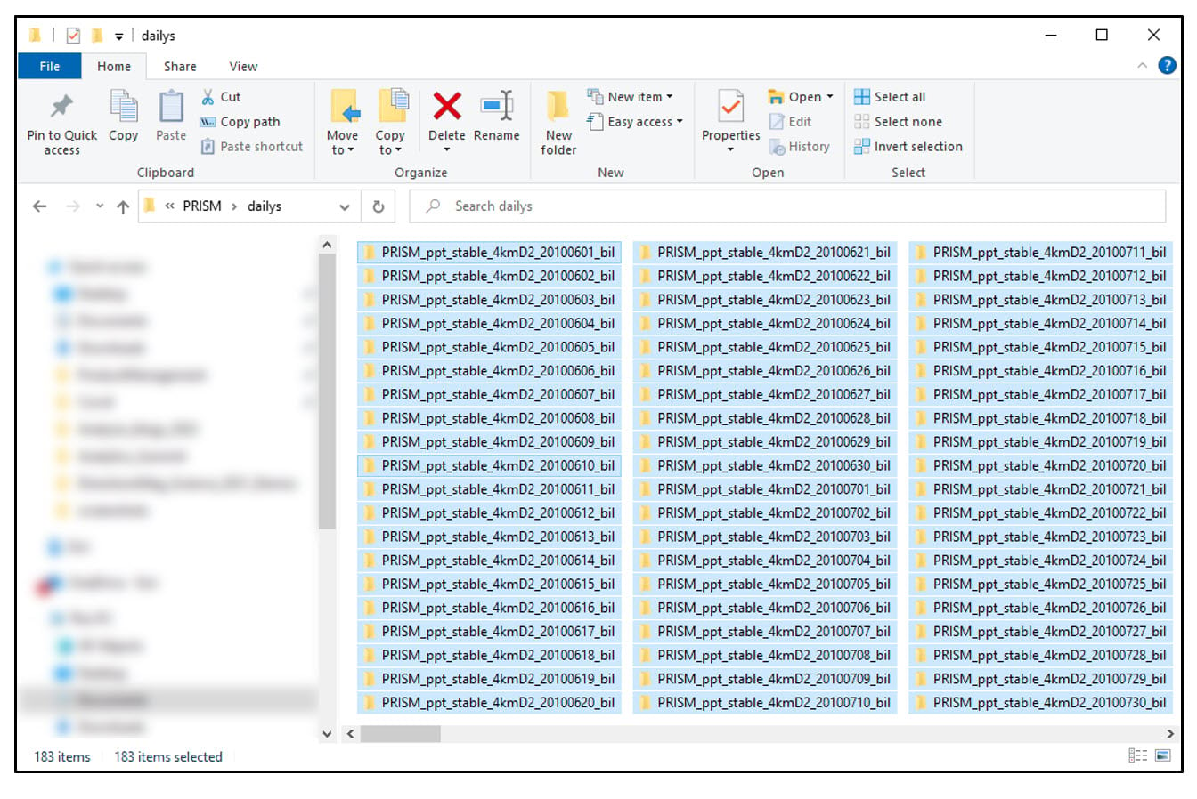
Within this function, you can specify the start and end date of the download period. I knew that downloading and processing ~11,000 rasters at once would not be manageable on my machine (or within R, period), so I would have to download the data and process it in batches. After a bit of testing and experimentation, it appeared that roughly 200 or less rasters in each batch would be a workable size. This combined with the fact that each of the precipitation variables is calculated for every season in the 30-year time series, led me to the following pattern for determining the start and end date of each batch:
- Winter: December 1 to February 28* = 89 or 90 daily rasters
- Spring: March 1 to May 31 = 91 daily rasters
- Summer and Fall**: June 1 to November 30 = 182 daily rasters
For the purposes of this study, the 30-year time series started on December 1, 1981 (winter 1981) and ended on February 28, 2011 (winter 2010). That means the following processing steps would need to be performed on 90 individual batches (30 winters + 30 springs + 30 summer/fall combinations).
Data engineering: Cleaning and wrangling
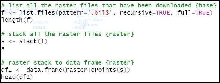
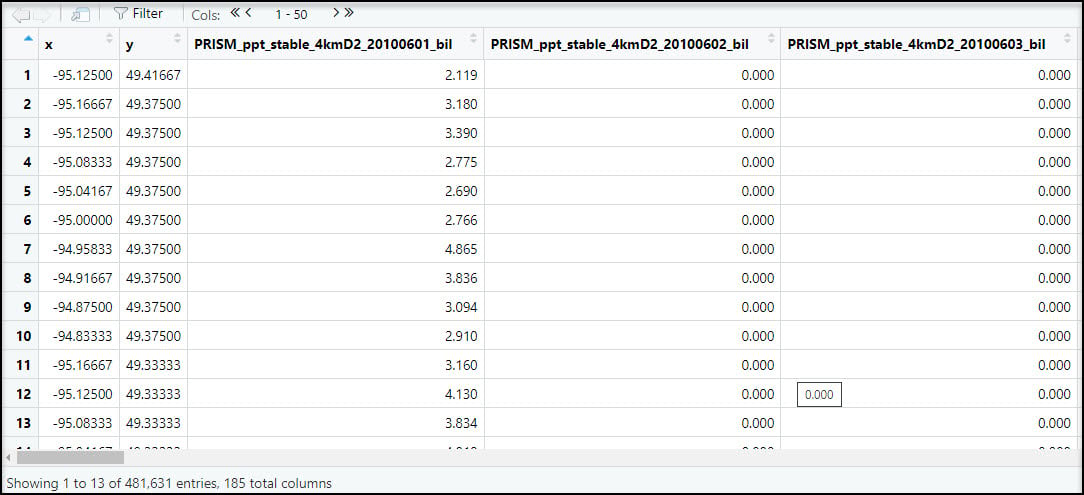
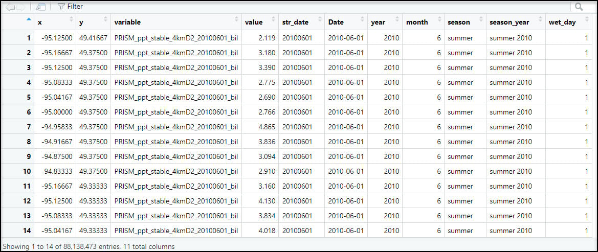
Because our end goal is to have a dataset with 16 precipitation variables at each location, we need to get our data in tabular format. This was achieved by first using the stack function to combine the rasters into one RasterStack object, then converting the RasterStack to a data frame via the rasterToPoints function. The result is a data frame of 481,631 locations by 185 columns (for one summer/fall batch), with two columns representing the x/y coordinates of each location, and the remaining columns representing the total precipitation (mm) for each day in the time series.
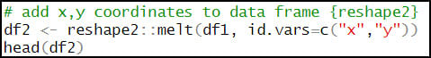
Next, we’ll use the melt function to flip the table from wide (481,631 rows x 185 columns) to long (88.1 million rows x 4 columns), so now the rows contain the entire time series of precipitation at each location. Note that the “variable” column contains the file name of each input raster.
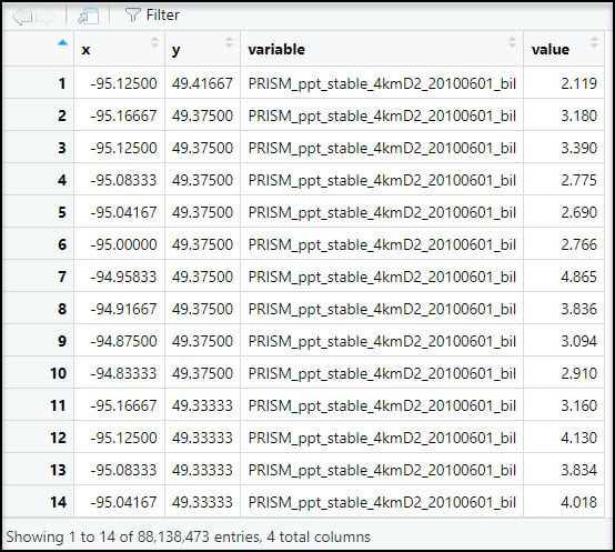
Eventually, we’ll be calculating the seasonal averages of several precipitation variables, so we need a way to assign seasons to each data point. To do this, we’ll use the substr function to extract the date information based on index positions in the “variable” column and insert it into a new column “str_date”.

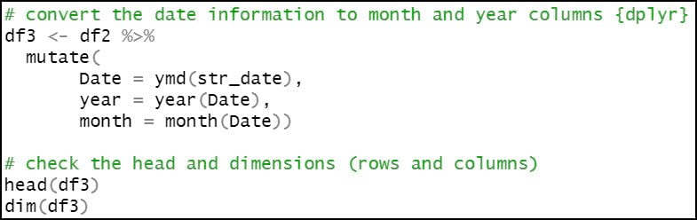
We then use the mutate function four separate times to engineer a series of new variables based on existing variables in the dataset.
- Convert the date information to month and year columns.
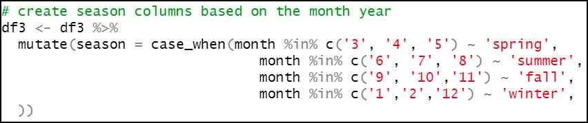
- Create a new “season” column, which assigns the months of the year to seasons, following the pattern below:
-
- Spring – March, April, May (3rd, 4th, 5th months of the year)
- Summer – June, July, August (6th, 7th, 8th months of the year)
- Fall – September, October, November (9th, 10th, 11th months of the year)
- Winter – December, January, February (12th, 1st, 2nd months of the year)
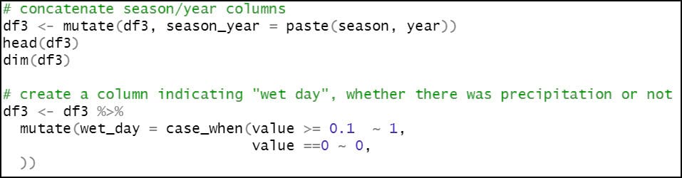
- Concatenate the “season” and “year” columns, so that we can calculate our seasonal averages for each year.
- Create a new boolean column “wet_day”, which indicates whether each location experienced precipitation on a particular day. In this case, a location is considered a “wet day” and assigned a value of 1 if it received greater than or equal to 0.1 mm of precipitation in a day, and 0 if less. This indicator column will be used in subsequent steps to calculate the precipitation variables that measure variability across a season.
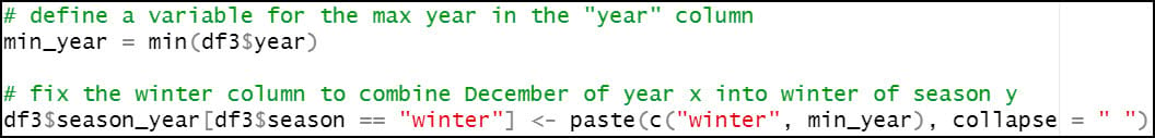
As noted in the section above, the winter season ranges from December 1 of year y to February 28 of year y+1. As such, we need to ensure that for every time this script runs, any data point in January or February is reassigned to the previous year. For example, January and February 1982 actually belong to the winter season of 1981. So here, if the “season” column contains “winter”, we update it with the previous year. Otherwise, the “season” column remains the same.
Data engineering: Creating the seasonal precipitation variables
The next step and perhaps the most important one in the workflow is creating the seasonal precipitation variables. For this, we’ll rely on the aggregate function three separate times to create three new data frames. This function is very useful for calculating summary statistics on subsets of data.
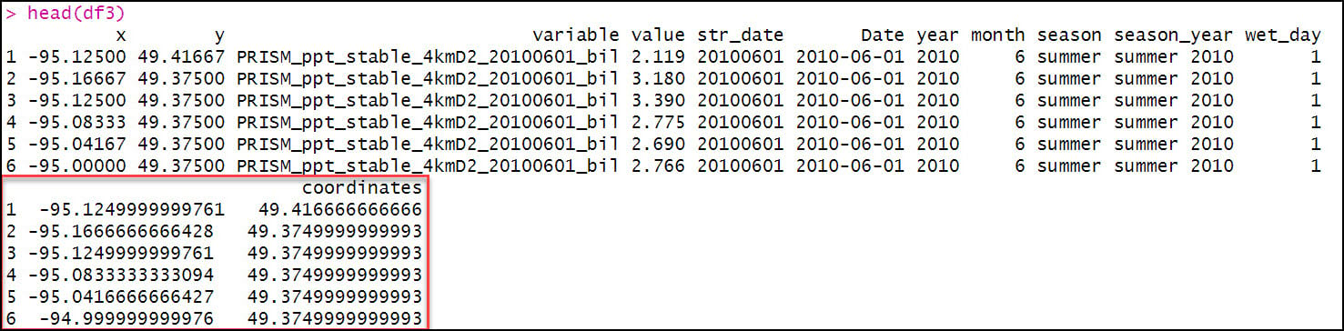
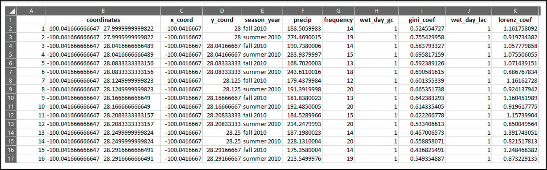
First, however, we need to use mutate one more time to concatenate the x/y columns into a new “coordinates” column to ensure that each location has a unique identifier.

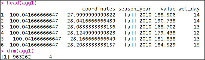
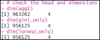
The first aggregation calculates the total precipitation (“value”) and total precipitation days (“wet_day”) within a season (“season_year”) for each location (“coordinates”) in the dataset. The FUN argument specifies the summary statistic that is applied to each subset (location/season pair), which in this case is sum to get the total precipitation (mm) and total days with precipitation in a season.

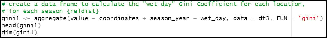
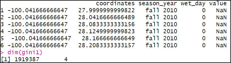
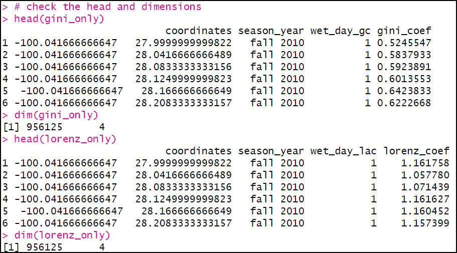
The second aggregation calculates the Gini Coefficient of precipitation within a season for each location. Note here that “wet_day” is included in the aggregation because the Gini Coefficient calculation only includes days when precipitation occurred. The FUN argument here calls the gini function from the {reldist} R package.
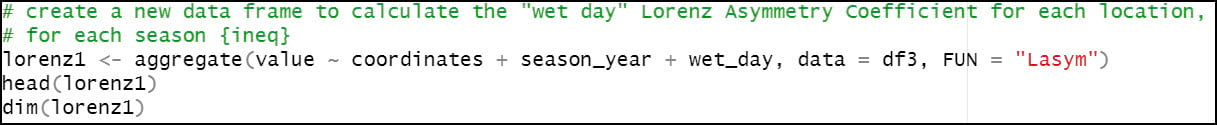
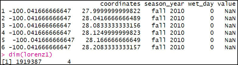
The third aggregation calculates the Lorenz Asymmetry Coefficient of precipitation within a season for each location. Like the Gini, “wet_day” is included in the aggregation because the Lorenz Asymmetry Coefficient calculation also only includes days when precipitation occurred. The FUN argument here calls the Lasym function from the {ineq} R package.
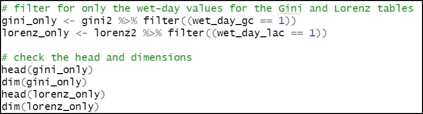
After a few more lines of code to rename columns to make them more understandable, we now have three separate data frames containing our calculated precipitation variables. Because we know that the Gini and Lorenz Asymmetry Coefficients can only be calculated on days when precipitation occurred, we use the filter function to return rows that meet a condition, in this case “wet_day” = 1.
We’ll then join these three separate data frames together using the merge function two times in a row. First, we join the Gini and Lorenz data frames together, then we join that result to the data frame containing the aggregated total precipitation and precipitation days attributes. Note that in both of these joins, the common attribute (key field) is actually a combination of the “coordinates” and “season_year” columns, because there are precipitation variables for two seasons for each location.
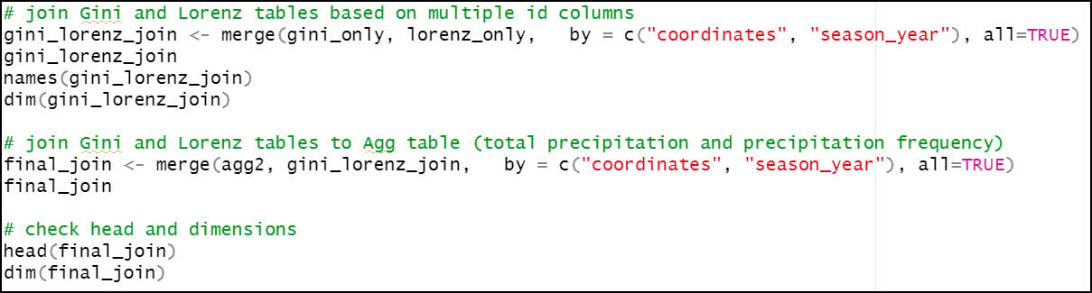
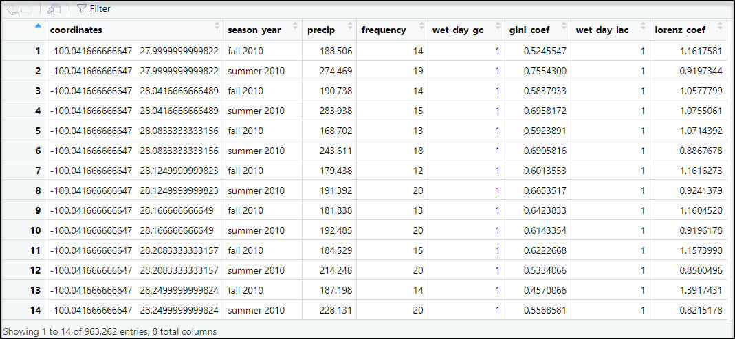
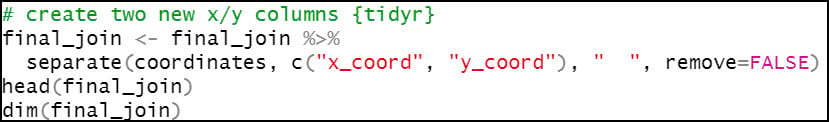
Because we will eventually want to map and perform spatial analysis on this data within ArcGIS, we’ll use the separate function to split the “coordinates” column into individual columns representing the x- and y-coordinate for each location.
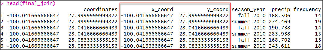
Last, we’ll write out the final joined precipitation dataset as a CSV file that can then be used in ArcGIS, or in other data science and analytics software.

Final thoughts
Remember, the entire workflow described above only focused on two seasons (Summer and Fall, 2010). As mentioned above, it was necessary to perform this workflow in batches not only because of computer processing limitations, but more importantly because the precipitation variables are seasonal calculations based on daily precipitation data. That means that within the 30-year time series covered by this study, there were a total of 120 seasons. Because I was able to process the summer and fall seasons together, this amounted to 90 batches that I had to run manually. Fortunately, I was able to automate much of this process using R, including the downloading of each batch of rasters, all the cleaning/wrangling/engineering steps, writing out of the final CSV, and deletion of each batch of rasters. The only thing I had to change with each batch was the start and end date of the batch. The final result was a folder containing 90 CSV files, one for each batch. Each CSV file contains the final calculated precipitation variables for each location, for a given season.
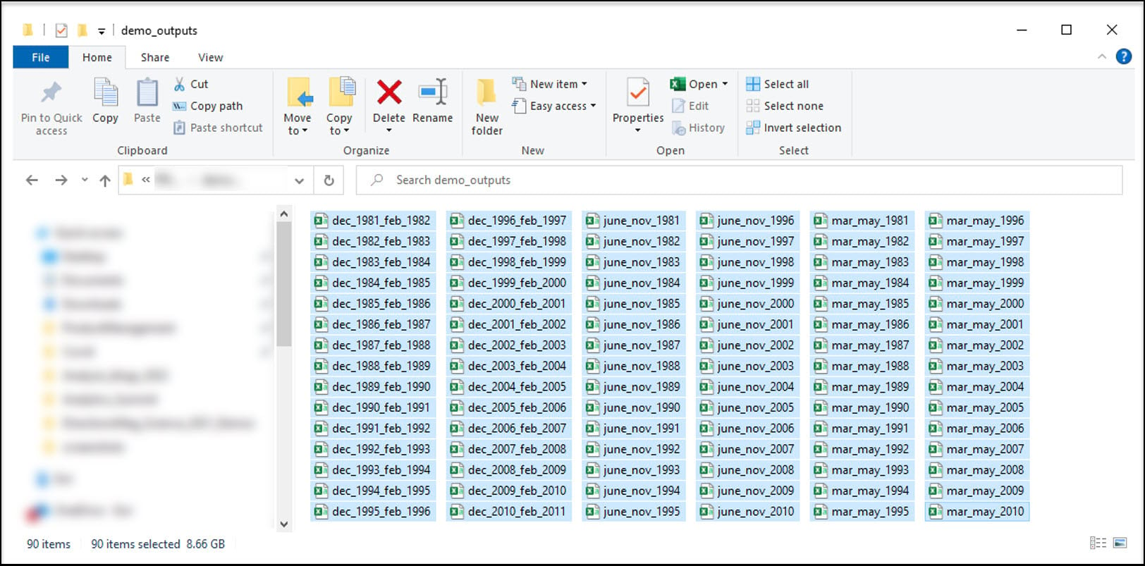
Here are some rough estimates of the amount of time it took to perform this workflow on all 90 batches.
- Winter season processing (89 or 90 daily rasters) = ~24 minutes x 30 batches = ~12 hours
- Spring season processing (91 daily rasters) = ~25 minutes x 30 batches = ~12.5 hours
- Summer/Fall season processing (182 daily rasters) = ~45 minutes x 30 batches = ~22.5 hours
So all told, it took nearly 50 hours of running R code to get to the point where I have this folder of CSV files (and that doesn’t include actually writing the R code to do it). Ever hear that phrase “data engineering takes up 80% of your time in a data science project”??
Guess what…we aren’t even close to being done. Jump to the next blog article to learn how we’ll process all of these CSV files into our final, analysis-ready dataset.


Article Discussion: