Introduction
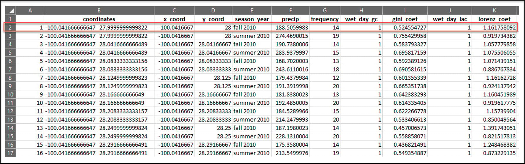
In the previous blog article, we used R to process a 30-year daily precipitation dataset (~11,000 rasters) into a collection of 90 CSV files, where each CSV file contains seasonal calculations of four precipitation variables at each location in a 4km by 4km gridded dataset of the US. For example, the x/y location in the first row of this CSV file experienced precipitation in 14 of the 90 days in the Fall of 2010, totaling about 188 millimeters of precipitation.
In this blog article, we’ll use Python* to do some additional data engineering steps to further aggregate the data by calculating the long-term, 30-year averages of each of the four precipitation variables, for each season. Our final dataset will therefore contain 16 precipitation variables for each location in the 4km by 4km grid.
Python libraries
Just as we did in the previous blog post, our first few lines of code will be for loading the Python libraries we require for our task.
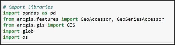
- pandas – working with and manipulating tabular data
- arcgis – the ArcGIS API for Python, used to convert ArcGIS data to Pandas DataFrames
- glob – working with file paths
- os – working with operating system files and file directories
Combining multiple CSVs into one Pandas DataFrame
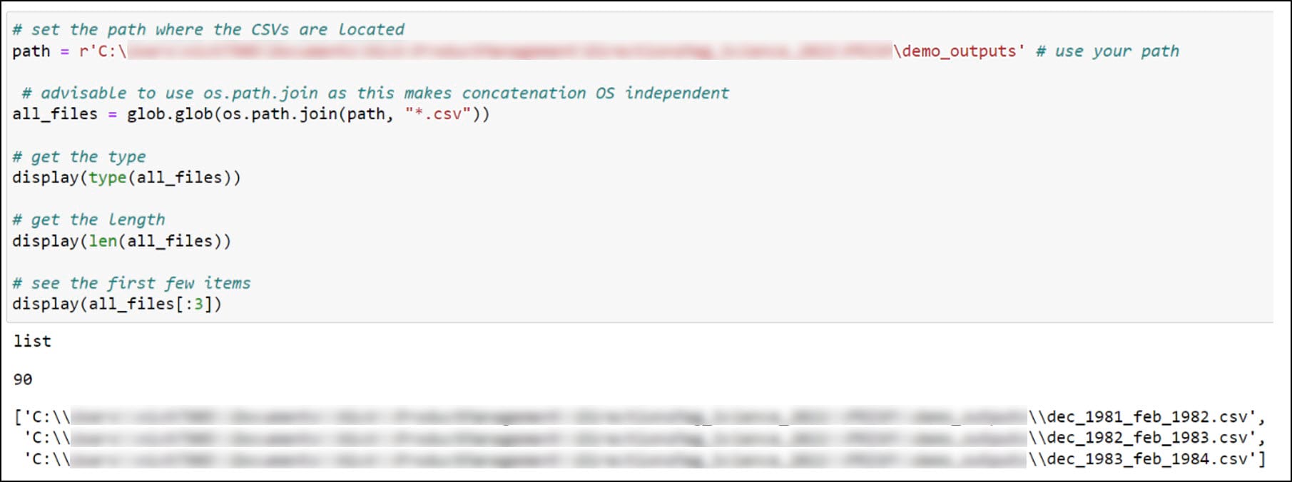
The first thing we need to do is have a look inside the folder of CSVs we created in the first blog. We’ll create a variable for the folder location where the CSVs are stored, then use the glob library to search for files in this folder location that match a certain pattern, in this case all files that end with a .csv file extension. The result is stored as a list with 90 elements representing the 90 seasonal CSV files.
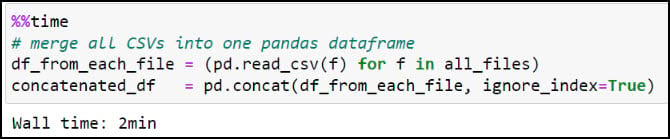
Next, we’ll use the Pandas .read_csv function in a Python list comprehension to read each CSV file into a Pandas DataFrame, then use the pandas .concat function to combine all 90 DataFrames into one large DataFrame.
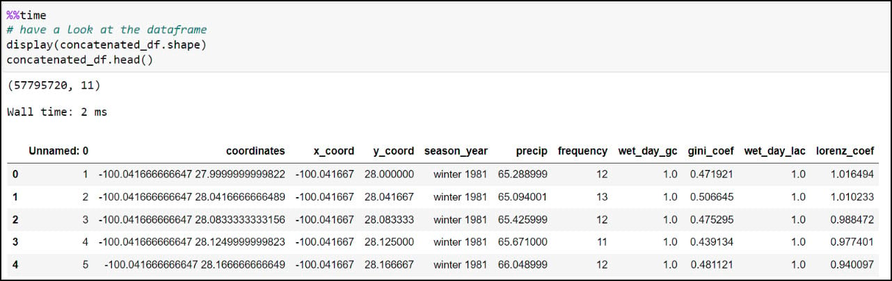
We can have a look at the dataset dimensions (rows and columns) using the .shape property, then use the .head function to look at the first few rows of the DataFrame. You should recognize the precipitation variables from the columns in the CSV files, then double check that the total of 57,795,720 rows corresponds to the 30-year seasonal time series at each location (481,631 locations * 120 seasons).
Last, let’s make sure we get a sense of whether we have any missing data. For this, I’ll use the .isnull function to find missing values in the DataFrame, then the .sum function to add them up for each row. In this case, the axis parameter indicates whether you are adding horizontally (rows) or vertically (columns).
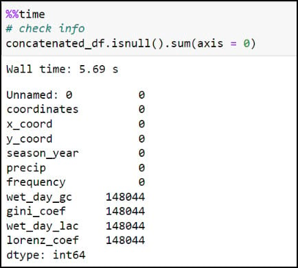
Here we can see that four of the columns contain about 0.25% missing values, which by most standards is negligible and will not have an impact on the final results. In our case, we know that these missing values are expected because they are locations that experienced zero precipitation throughout an entire season, and therefore will not have measures of variability (Gini Coefficient) or inequity (Lorenz Asymmetry Coefficient) within a season.
Data engineering: Calculating the 30-year averages of the four seasonal precipitation variables
At this point, we have a 120-season time series of each of the four precipitation variables at each location in this dataset, where the season is indicated by the “season_year” column. We ultimately want to calculate a single average of each of the precipitation variables for each season, at each location, so the resulting dataset will contain four seasonal averages (winter, spring, summer, fall) of each precipitation variable, at each location.
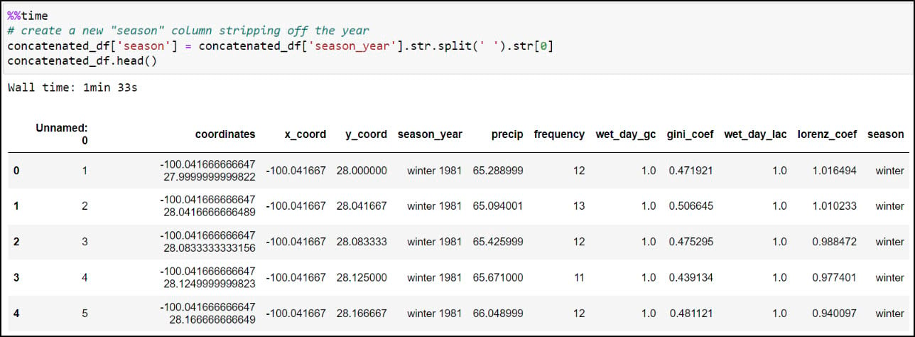
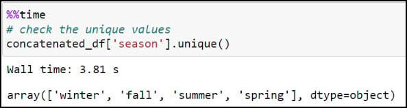
We’ll first create a new “season” column by stripping off the year from the “season_year” column. This is achieved using the .str.split function, which splits a text string based on a separator or delimiter (in this case, a space) and then returns the first index position, which here is only the season from the “season_year” column. We can then use the .unique function on the new column to verify that the four seasons are the only values available.
We now have what we need to calculate one single average for each precipitation variable, for each season, at each location. We’ll use .groupby to create groupings of data, then .agg to apply an operation to the groupings. In our case, we’re grouping the data by combination of location and season (e.g. four seasons at each location), then taking the averages of all four precipitation variables within each season. The .reset_index method at the end ensures that the DataFrame has a numeric index that starts at 0 and increases by 1 for each subsequent row.
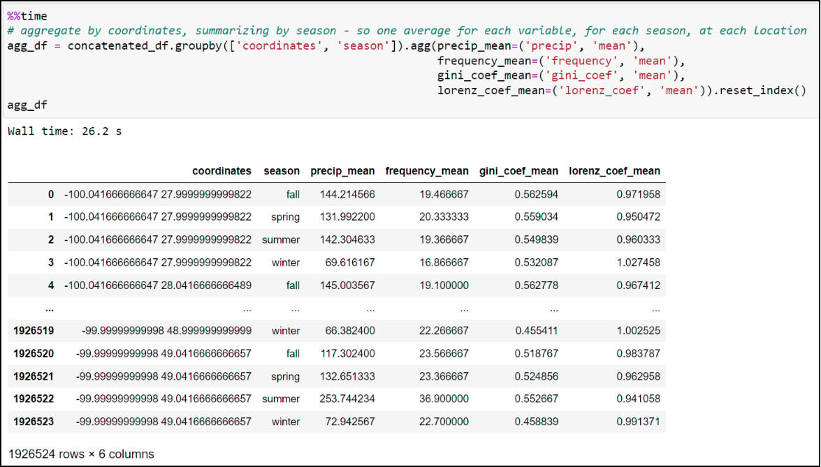
We can see here that the DataFrame has been reduced from 57,795,720 rows (4 seasons x 30 years x 481,631 locations) to 1,926,524 rows containing the average of each of the four precipitation variables, for each season, in each location (4 seasonal averages x 481,631 locations).
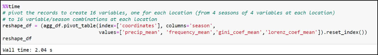
While this step has drastically reduced the number of rows in the table, it is still a long table, meaning that there is duplicate information in the table rows. In this case, there are four rows for each location (“coordinates” column), with each of these rows representing the seasonal average of the four precipitation variables. We’ll next use the .pivot_table function to flip the table from long to wide, such that each row represents an individual location and the columns contain the corresponding season/precipitation variable information. The index parameter specifies which column becomes the row index of the resulting DataFrame, which in this case is the “coordinates” column. We specify “season” in the columns parameter, and the values parameter contains the four precipitation variables. The resulting DataFrame now contains one row for each location and a total of 16 precipitation variables (4 variables x 4 seasons).
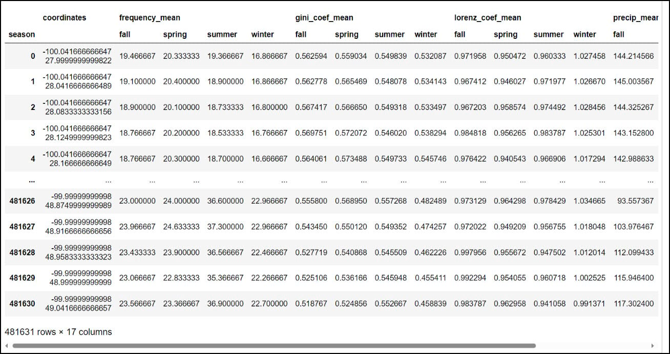
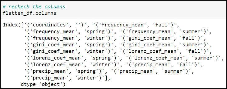
You might notice that the resulting DataFrame appears to have two header rows (the precipitation variable, with four seasons under it). The pivot table step actually results in something called a MultiIndex DataFrame (e.g. hierarchical index), which means that it can have multiple levels. In this example, the two levels are the precipitation variable and the season. We had to use one more step to flatten the multiindex, which we achieved by converting the Multindex DataFrame to a NumPy array, then back to a single index DataFrame using the .to_records function.
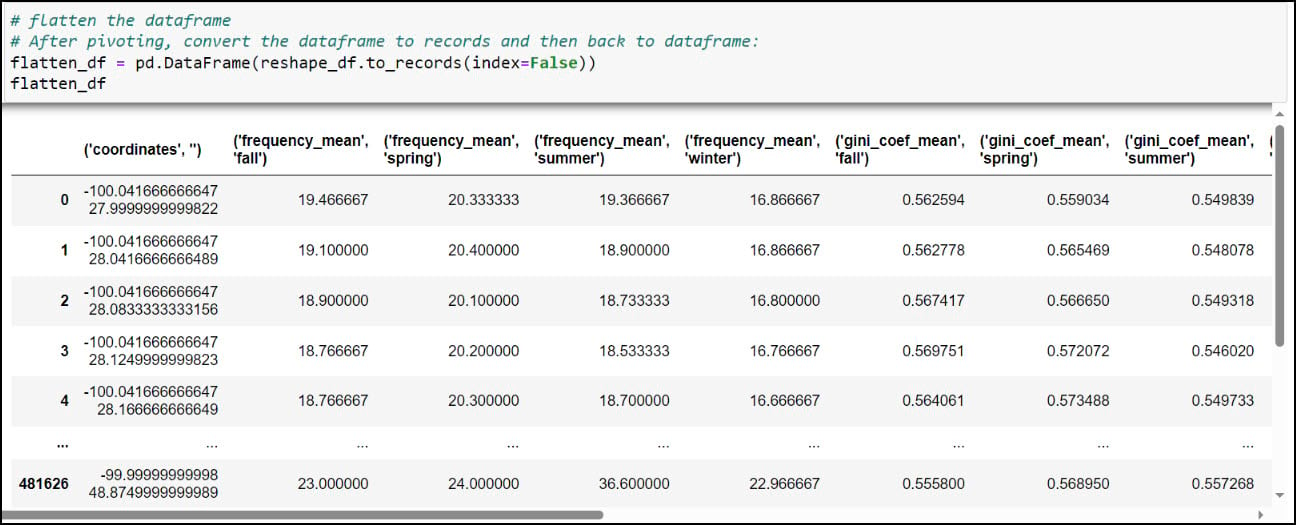
As you can see, the column names contain parentheses and single quotes, and it is always a best practice to remove such special characters. We can print all the column names using the .columns attribute, then pass a dict into the .rename function, where each key is the original column name mapped to each value as the new column name.
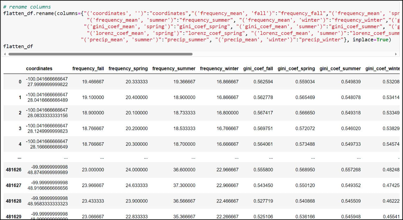
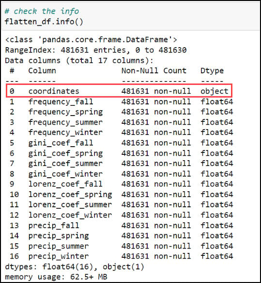
At this point, we have nearly everything we need to proceed with the next parts of our analysis. Each row in the DataFrame contains 16 columns representing 30-year seasonal averages of four different precipitation variables (4 seasons x 4 variables), along with a “coordinates” column indicating one of the 481,631 locations in the dataset. Obviously, this is the column that we’ll use to get this information on the map, but there are a few more simple yet crucial steps we have to do first.
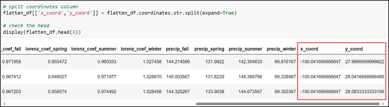
The first step is to create two new columns representing the x- and y-coordinates of each location. Recall earlier in this blog that we used the .str.split function to split a text string based on a separator or delimiter, and we’ll do the same thing again here to split the values in the “coordinates” column based on the space between them. This results in two new individual columns, “x_coord” and “y_coord”.
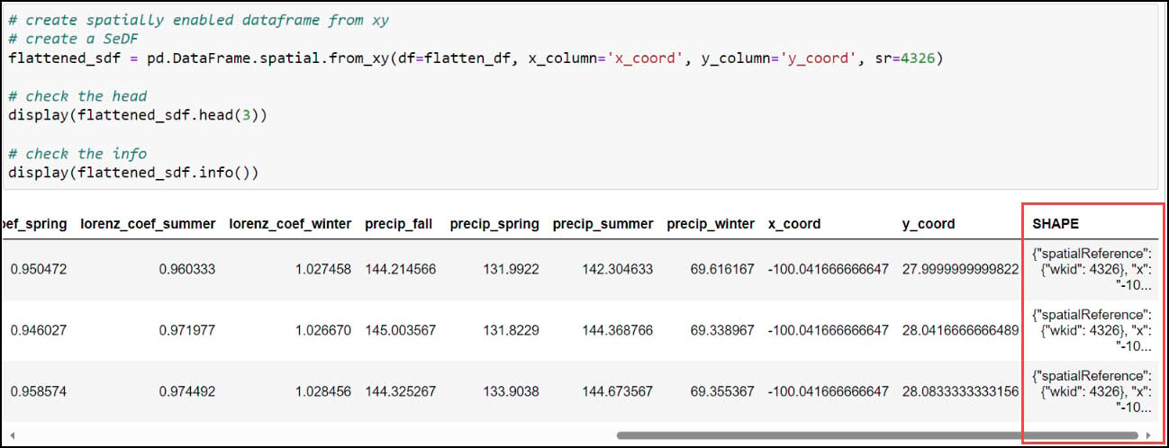
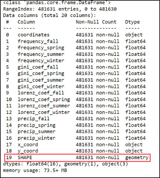
With our x- and y-coordinates now in their own columns, we can use the ArcGIS API for Python to convert the DataFrame into a Spatially Enabled DataFrame (SeDF). A SeDF is essentially a Pandas DataFrame with an additional SHAPE column representing the geometry of each row. This means that it can be used non-spatially in traditional Pandas operations, but can also be displayed on a map and used in true spatial operations such as buffers, distance calculations, and more.
Here, we pass the DataFrame into the .from_xy method on the ArcGIS API for Python’s GeoAccessor class, specifying “x_coord” and “y_coord” as the x- and y-columns, respectively, as well as the appropriate coordinate system.
Last, we’ll use the ArcGIS API for Python’s .to_featureclass method to export the final, cleaned SeDF as a feature class in a geodatabase so we can use it in further analysis in ArcGIS Pro.

Final thoughts
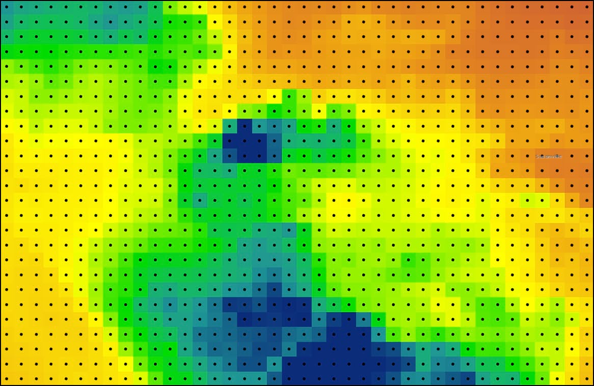
At this point, we now have a feature class that represents a gridded point dataset covering the contiguous United States. Each of the 481,631 grid points corresponds to the raster cell centroid of the original 4km by 4km PRISM precipitation dataset.
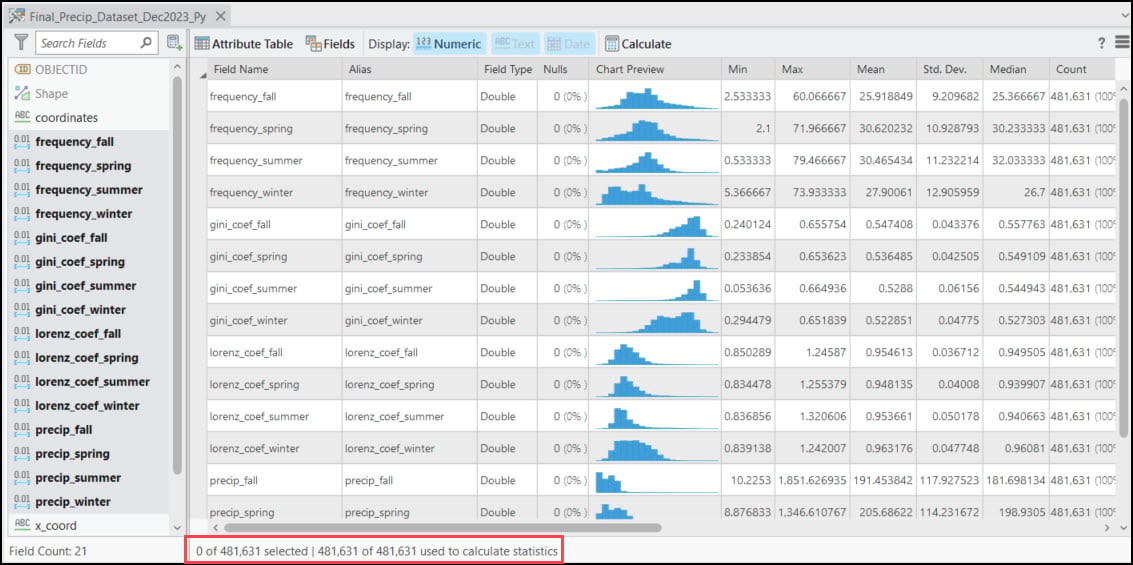
Each of these points also contains 16 columns representing the 30-year seasonal averages of the four precipitation variables calculated in Blog #2 in the series. Using ArcGIS Pro’s Data Engineering view, we can see and explore the summary statistics and distributions of each variable in the feature class.
Appendix
Or if you prefer… do it in R!
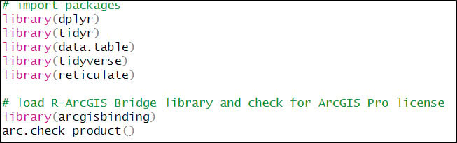
1. R packages
-
- {dplyr} – working with and manipulating data frames
- {tidyr} – creating “tidy” data (cleaning, wrangling, manipulating data frames)
- {data.table} – working with data frames
- {tidyverse} – collection of R packages for data science
- {reticulate} – provides interoperability between R and Python, allowing you to call Python functions from within R scripts. This allows you to call ArcPy geoprocessing tools from within R, for example.
- {arcgisbinding} – the R-ArcGIS Bridge, which connects ArcGIS Pro and R
2. Combine all CSV files into one R data frame
- list.files – returns a list of all files or directories at a specified path
- %>% is a pipe operator, which makes it easy and efficient to chain multiple functions together in R. The input of each successive function is the output of the previous function. Here, the list of 90 CSVs is piped into the lapply function, which is used to apply a function over a List or Vector in R. In this case, the read_csv function is applied to each of the 90 CSV files in the list and converts it to a tibble, which is a modern version of the R data frame. The 90 tibbles are then piped into the bind_rows function, which is used to bind (combine) many data frames into one.
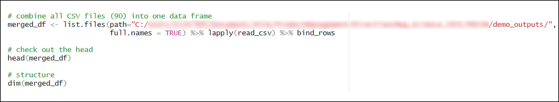
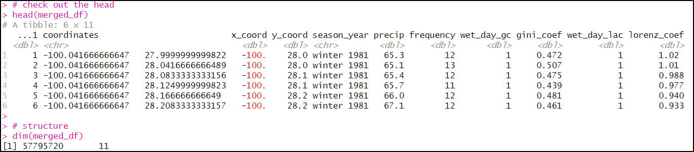
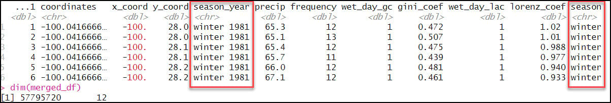
- The final combined data frame has the expected 57,795,720 rows (120 seasons x 481,631 locations) and 11 columns.
3. Data engineering and wrangling
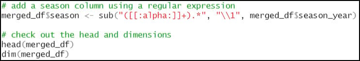
- Create a new “season” column that includes only the season (not year) from the “season_year” column. This requires use of the sub function, which is used to replace one string with another. In the code below, we’re using a regular expression within the sub function to replace a text string pattern (e.g. “winter 1981”) with only the first word in the text string pattern (e.g. “winter”) and then populate a new “season” column with this value.
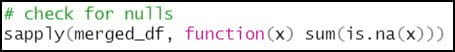
- Check for null values. We use sapply to apply a function that identifies nulls (is.na) and then totals (sum) the missing values for each column in the data frame.

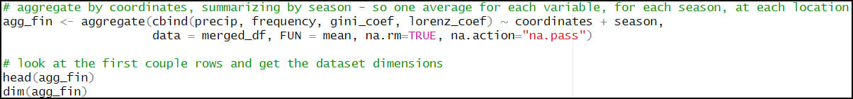
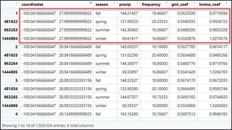
- Calculate one single average for each precipitation variable, for each season, at each location. For this, we’ll rely again on the aggregate function to help us calculate summary statistics on subsets of data. Here, we calculate the average precipitation (“precip”), average number of precipitation days (“frequency”), average Gini Coefficient (“gini_coef”) and average Lorenz Asymmetry Coefficient (“lorenz_coef”) for each of the four seasons, at every location in the dataset. The FUN argument specifies the summary statistic that is applied to each subset (location/season pair), which in this case is the mean.
- Calculating the seasonal averages of each of the four precipitation variables reduces our data frame from 57,795,720 rows (481,631 locations x 4 seasons x 30 years) to 1,926,524 rows (481,631 locations x 4 seasonal averages at each location).
- Flip the table from long to wide, such that each row represents one location, and the four seasonal averages for each of the four precipitation variables become the columns. Here we use the dcast function to reshape the data frame, which is essentially the same as using .pivot_table with Pandas in Python. In the formula parameter, the left-hand side specifies the variable you want to pivot on and keep as the row index (e.g. “coordinates”) and the right-hand side represents the variable you want to pass to the rest of the columns (“season”). In other words, instead of each location having four rows for each season and four columns for the precipitation variables, the output data frame will have one row for each location and 16 columns, one for each season/precipitation variable combination.

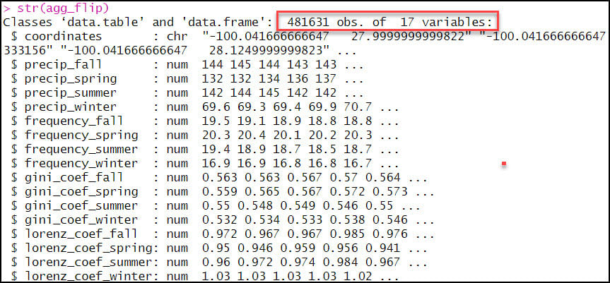
- As expected, the output data frame contains one row for each of the 481,631 locations, with 17 columns representing the location coordinates plus 16 precipitation variables.
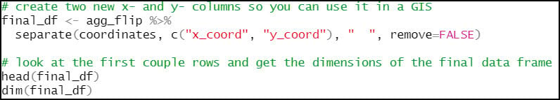
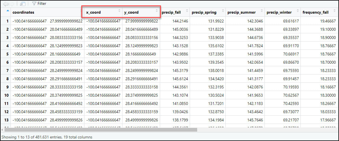
- As we did in the first blog in this series, we’ll again use the separate function to split the “coordinates” column into two new columns representing the x- and y-coordinates for each location individually.
4. Export data for further analysis in ArcGIS using the R-ArcGIS Bridge
- Last, we’ll use the R-ArcGIS Bridge {arcgisbinding} package to convert our R data frame to a feature class within a file geodatabase. The arc.write function allows you to export several different R objects (data frames, spatial {sp} and {sf} objects, {raster} objects, etc.). In our case, we’ll pass in the R data frame, specify the x- and y-coordinate columns in the coords parameter, and pass in “Point” type and the appropriate spatial reference into the shape_info parameter. This last step creates a new file geodatabase feature class that we can use for further analysis in ArcGIS Pro.


Article Discussion: