Introduction
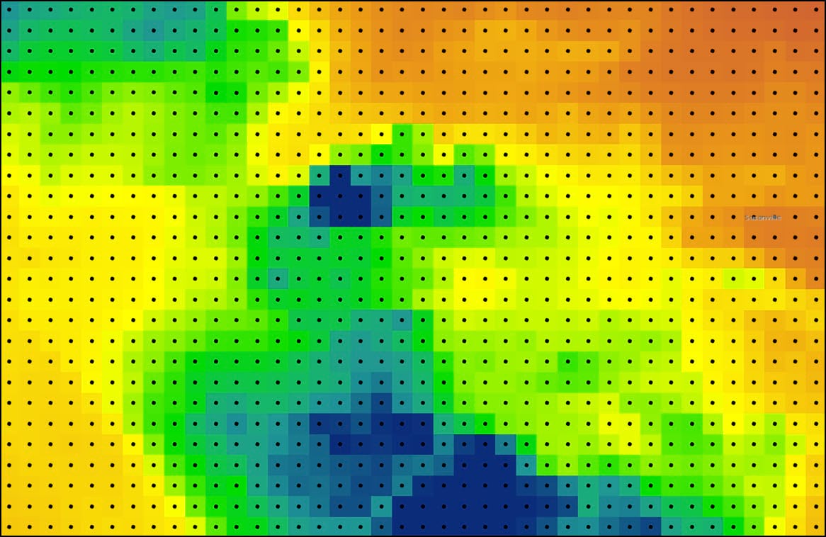
In the previous blogs in this series, we used a combination of R and Python to access, clean, wrangle, convert, engineer, and otherwise transform a 30-year time series of ~11,000 daily precipitation rasters into one feature class containing 16 different seasonal precipitation-related variables. The final feature class is a gridded point dataset covering the contiguous United States. Each of the 481,631 grid points corresponds to the raster cell centroid of the original 4km by 4km PRISM precipitation dataset.
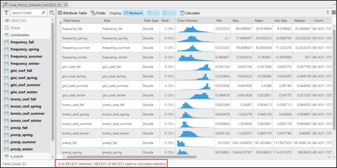
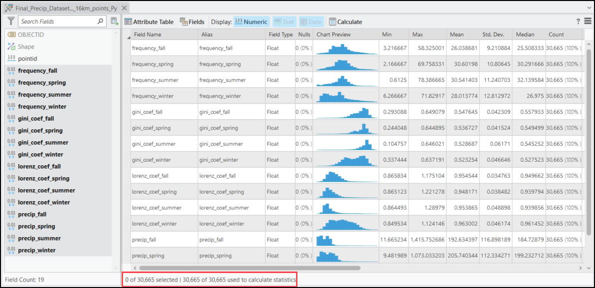
Each of these points also contains 16 columns representing the 30-year seasonal averages of the four precipitation variables calculated in Part #2 in the blog series. Using ArcGIS Pro’s Data Engineering view, we can easily see and explore the summary statistics and distributions of each variable in the feature class.
Now to the fun part…spatial analysis!
Post-processing and spatial aggregation
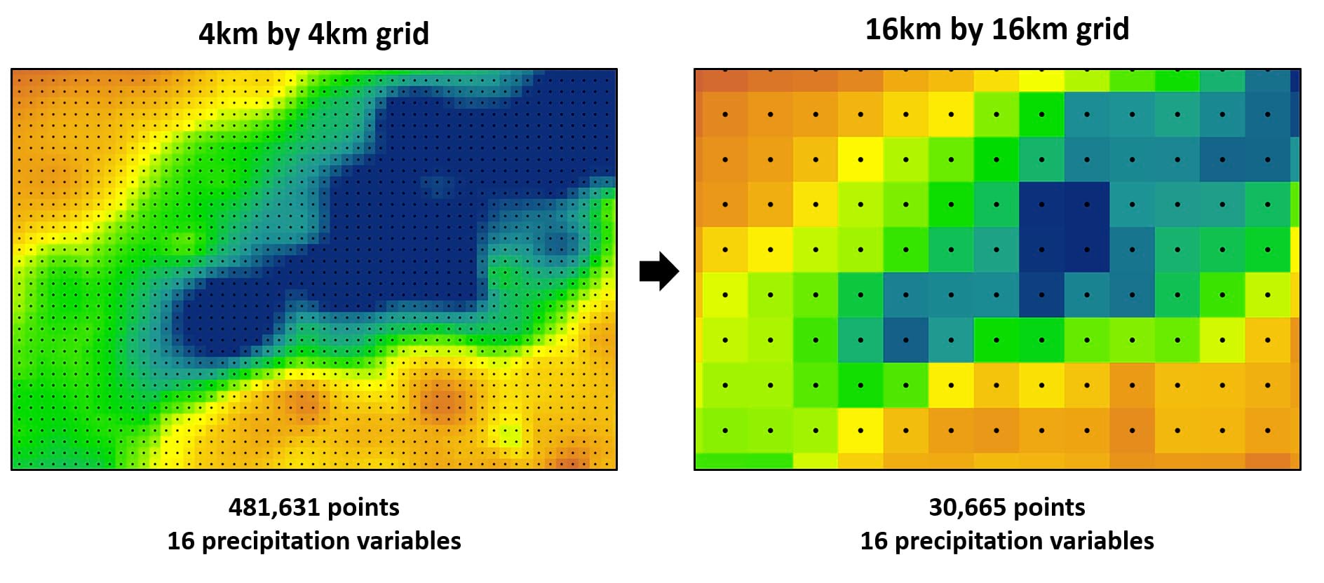
If we refer back to the overall workflow graphic shown in Part #1 of this blog series, you’ll note that the third section “Data Post-Processing” involves a spatial aggregation step. The idea here is to coarsen the dataset (e.g. reduce the resolution) to remove noise and make it easier to work with later in the workflow. In our case, we need to spatially aggregate the gridded dataset by averaging all 16 precipitation variables from a 4km by 4km grid to a 16km by 16km grid. At the granular level, this means taking the spatial average of 16 grid points and creating a new grid point at their centroid.
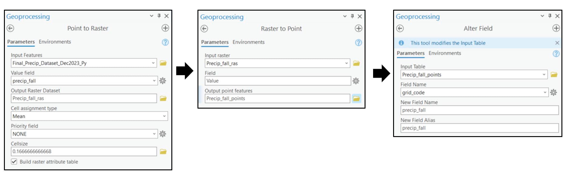
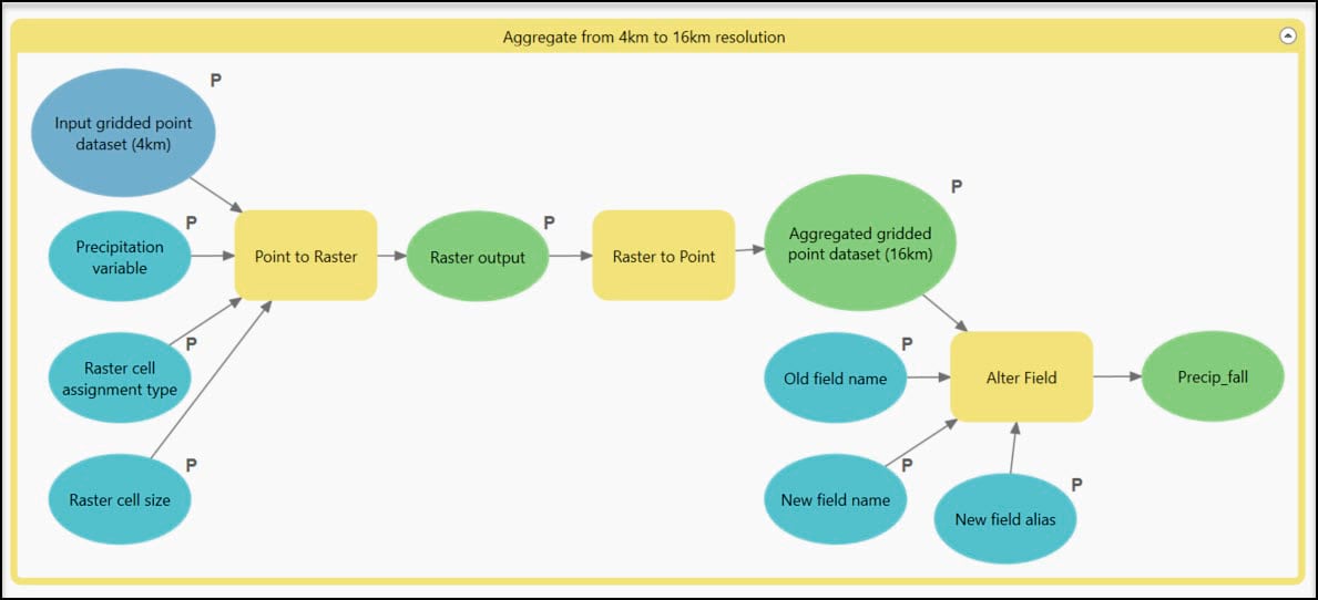
In ArcGIS Pro, this spatial aggregation process involves three geoprocessing tools:
- Point to Raster – converts the 4km grid points to a raster, where we can specify the cell size. In our case, we specify 0.166 to represent a 16km by 16km raster cell. The Value field parameter specifies the attribute value to aggregate (e.g. one of the 16 precipitation variables). The Cell assignment type parameter specifies which value will be given to each new raster cell based on the underlying points being aggregated, which in our case is the spatial average (mean) of each group of 16 grid points.
- Raster to Point – converts the 16km by 16km raster dataset back to points, for the given precipitation attribute.
- Alter Field – used to rename fields in a feature class.
Using the 481,361 row, 4km gridded points dataset as our input, we run the three tools in succession and end up with a 16km gridded points dataset containing 30,665 locations. Easy enough right?
Not so fast! Remember we have 16 precipitation variables to work with, so we need to run the three tools 16 different times each. That equates to 48 individual geoprocessing tool runs, and all the accompanying steps: open the tool, fill out the parameters, run the tool, close the tool, then repeat 47 more times. There has to be a better way, right?
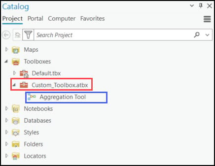
Automation opportunity #1: ModelBuilder
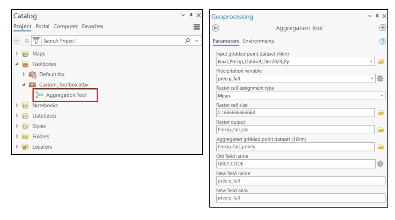
Running a series of geoprocessing tools in sequence is a perfect opportunity to use ModelBuilder. To do so, I’ve created a new toolbox in the Catalog pane and within it, a new blank model. In the model view, I’ve dragged and dropped my input layers and the three geoprocessing tools I need, did a bit of renaming and reformatting, and then strung them all together through a series of connections. I’ve also created variables (blue ovals) from several of the tool parameters so I can specify which values I want to use in the tools. Last, I can right-click on each of the model variables to flag them as model parameters so that they are exposed as geoprocessing tool parameters and behave as such after the model is saved. I can then open the model as a tool from within the Geoprocessing pane, interactively input the desired data and parameters, and run it like any other tool.
It’s incredibly easy, helpful, and certainly a time saver to run a model as a tool. However, it can only run the three geoprocessing tools on one precipitation variable at a time, so that means I need to run it 16 times. Another opportunity to automate!
Automation opportunity #2: Python
This time we’ll automate using some fundamental Python coding patterns and techniques. As such, we will transition our work back to the ArcGIS Notebook directly in ArcGIS Pro.
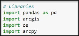
First, let’s get set up by importing our necessary Python libraries.
- pandas – working with and manipulating tabular data
- arcgis – the ArcGIS API for Python, used to convert ArcGIS data to Pandas DataFrames
- os – working with operating system files and file directories
- arcpy – the ArcGIS geoprocessing framework. Provides Pythonic access to the ~2,000+ geoprocessing tools, as well as functions for data management, conversion, and map automation
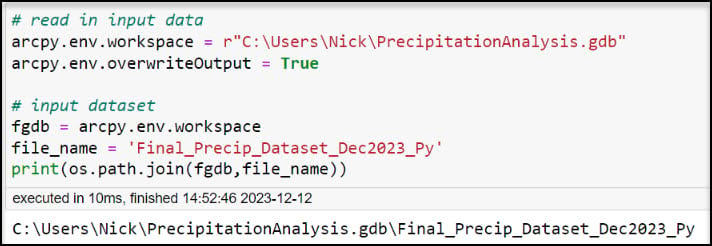
Next, we need to access our gridded dataset so that we can work with it in the Notebook. In a notebook cell, we can set the Current Workspace to be the geodatabase that contains all of our geoprocessing inputs and outputs. Environment settings such as this will now be honored by all subsequently run geoprocessing tools, regardless of their specific functionality. We can also set the overwriteOutput environment setting to True so that we can overwrite all geoprocessing outputs and don’t have to create a new file each time we run a tool.
We can create variables for the file geodatabase and the file name of the gridded dataset, then run the cell.
Because we need to run our geoprocessing model tool repeatedly (e.g. 16 times, once for each precipitation variable), let’s think of how to do this Pythonically. In other words, how can we use Python code to iterate over a function repeatedly?
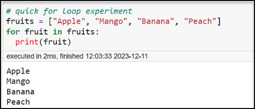
One of the most common ways to perform this type of task in Python is using a “for loop”, which is a block of code that is repeated a specified number of times. The number of times is dictated by the elements of an iterable object, e.g. items in a list, characters in a string, key/value pairs in a dictionary, etc.). Take this quick example from LearnPython.com:
Here we have a list of different fruits. We create a for loop to iterate over each item in the list, then run the print function four times, once on each of the fruits in the list:
Now let’s apply this same logic to our automation task. Instead of the list of fruits, however, we’ll use a list of the 16 precipitation variables. Instead of the print function, we’ll use our Aggregation geoprocessing model tool.
First, we’ll use the ArcPy ListFields function to generate a Python list of all the attribute fields in our gridded point dataset. In this example, we are using a Python list comprehension, which is essentially a for loop in a single line of code.
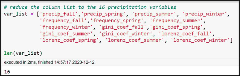
Because we only want to iterate over the 16 precipitation variables, we’ll create a new list excluding the OBJECTID, geometry, and other location-related fields.
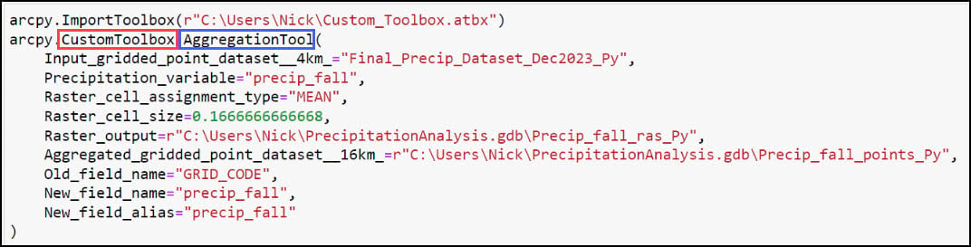
We’ll now take advantage of another powerful, yet overlooked functionality in ArcGIS Pro—the ability to copy the Python syntax from a geoprocessing tool.
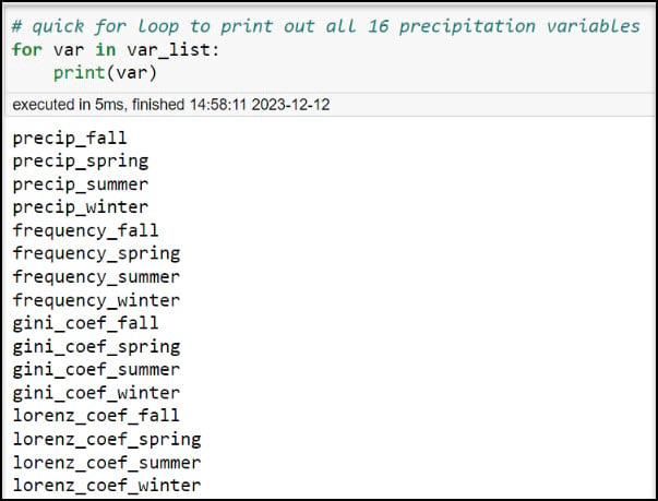
First, let’s make sure that we have a list that we can iterate over. We can create a quick for loop to print out each item in “var_list”.
Looks good! Now, we’ll open our Aggregation Tool and fill out the parameters as if we were going to run it one time. In the Run menu, you can select Copy Python Command to copy the syntax of the parameterized tool, then paste it into your Python scripting environment of choice.
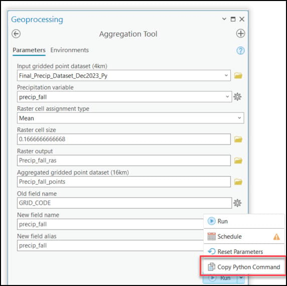
You can see from the code snippet below that the first line calls ArcPy’s ImportToolbox function, which is a requirement because we are using a custom toolbox. Below this, we can see the call to the Aggregation Tool in our custom toolbox, complete with all the parameters we filled out. If we were to now run this notebook cell, it would run the Aggregation Tool one time, in this case on one of the 16 precipitation variables—”precip_fall”.
However, we want to use a for loop to run the tool on each individual precipitation variable. In a new notebook cell below, copy the contents of the previous cell, then make the following changes:
- Insert the %%time magic command at the top of the cell to calculate the runtime of the cell.
- Insert comments about importing the custom toolbox and creating a for loop (optional).
- Above the Aggregation Tool syntax, insert a for loop to iterate over the list of the 16 precipitation variables.
- Indent the Aggregation Tool syntax such that it sits within the for loop.
- Replace the Input_gridded_point_dataset__4km_ parameter with the “file_name” variable, which is the 4km by 4km gridded dataset.
- Replace the hard coded values in the Precipitation_variable, Raster_output, Aggregated_gridded_point_dataset__16km_, New_field_name, and New_field_alias parameters with “var”. This will ensure that the for loop not only runs the Aggregation Tool 16 times, once for each precipitation variable in “var_list”, but that it also makes the corresponding changes to the new rasters and point datasets that are being created. For example, every new precipitation raster that is created will be named with the precipitation variable of interest and appended with underscores and the word “16km_ras_Py” (e.g. “precip_fall_16km_ras_Py”). The same concept applies to the output point files.
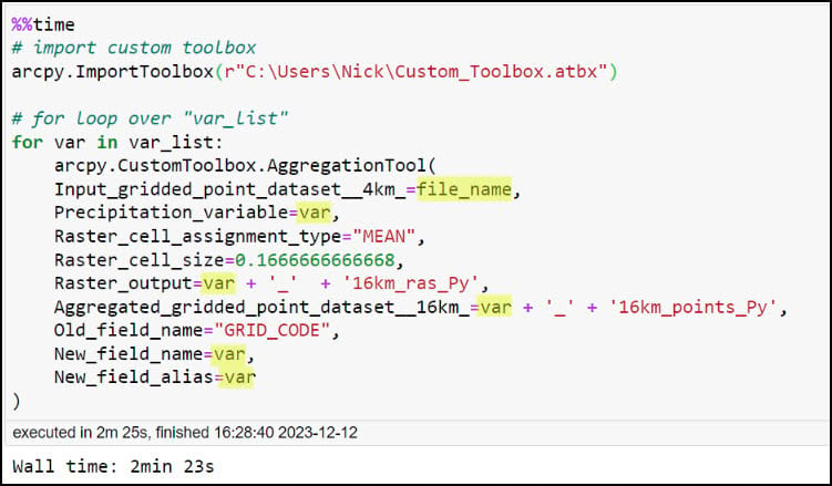
After running the notebook cell (and stepping away for a few minutes to stretch my legs), the loop completes having run the Aggregation Tool 16 times. Looking in my geodatabase, I see the output rasters and output point feature classes corresponding to each of the 16 precipitation variables.
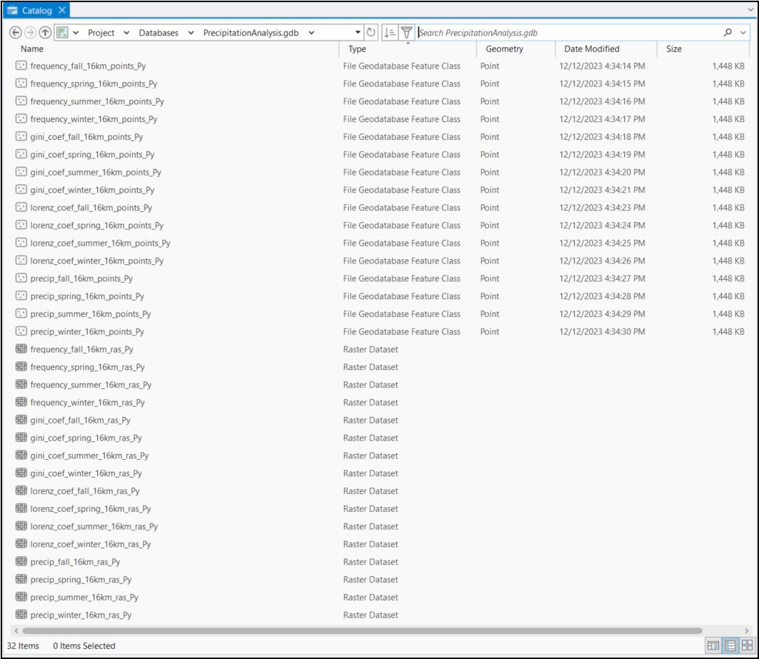
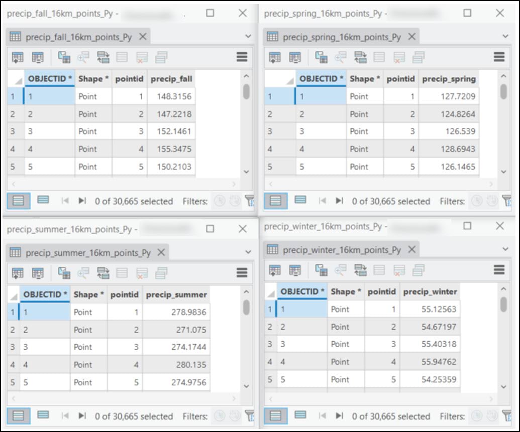
Each point feature class is a spatially aggregated version of the original 4km by 4km gridded dataset, representing a single precipitation variable in a 16km by 16km grid. The graphic below shows the Data Engineering view of four feature classes from the average precipitation variable, one for each season. Note that the schema is exactly the same in each feature class, including the “pointid” which represents a unique identifier.
To combine all 16 of these feature classes into one, we’ll use one more simple, yet powerful automation technique.
Automation opportunity #3: Batch geoprocessing
Batch geoprocessing is a way to repeatedly run a geoprocessing tool using either different input datasets or different parameter settings. Batch mode is available in many geoprocessing tools and can be accessed by right-clicking on a tool after you have searched for it or located it within a toolbox. In my case, I will be using the Join Field tool to join all 16 feature classes into one based on a common attribute, or “key” field.
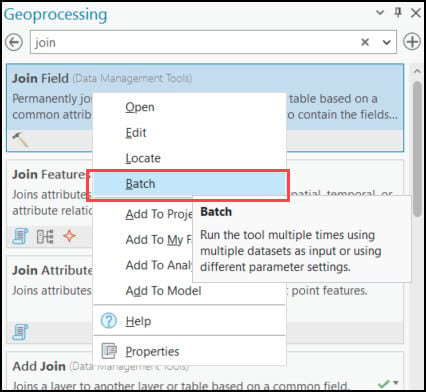
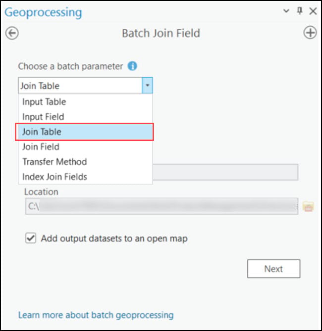
First, we’ll choose which parameter we want to batch. In this case, we are joining 15 feature classes to one, so we will choose Join Table. If we wanted to run this batch tool again, we do have the choice to save it, but for now we’ll just make a temporary tool.
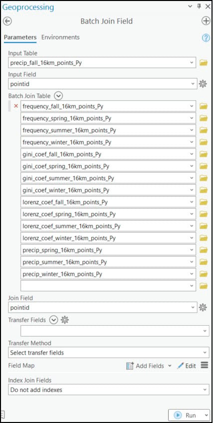
In the tool dialog, we’ll choose one of the 16 feature classes as the input table, select “pointid” as the unique identifier field on which the join will occur, choose the remaining 15 feature classes as tables to batch join, then choose “pointid” again as the key field for the join tables. Then click run and let the software do the work for you!
Last, we’ll use the Export Features tool to create a new feature class. Here, we can add and delete fields, rename them, and reorder them, amongst many other options. In our case, we are using this tool not to convert to a different format, but rather to clean up the dataset and get it ready for the upcoming analysis steps.
We can see from the Data Engineering view below that the final 16km by 16km gridded dataset contains the exact same schema as the original 4km by 4km dataset. However, because we have spatially aggregated from 4km to 16km, we’ve gone from 481,631 locations to 30,665 locations. This will be the input dataset to the upcoming machine learning steps. So let’s move on to the next blog!

Article Discussion: