Aboveground biomass is a crucial ecological variable for understanding the carbon cycle and assessing ecosystem productivities. Optical satellite remote sensing imagery, such as Landsat, proves invaluable in mapping land cover and identifying forest locations. Additionally, the altimeter sensors, like the Global Ecosystem Dynamics Investigation (GEDI), a lidar mission launched by NASA, provide vertical measurements of forests, enhancing our understand of the Earth. This blog aims to demonstrate how to map aboveground biomass by integrating remote sensing datasets from multiple satellite sensors and utilizing machine learning tools in ArcGIS Pro 3.2.
Workflow
Focusing on Oregon as a study area, the goal is to create an aboveground biomass map for the year of 2022 using a Random Tree regression model based on following multisource remote sensing data:
- GEDI Level 4A product: Trajectory point data from NASA’s GEDI mission containing aboveground biomass data.
- Landsat collection 2 from USGS: Includes the surface reflectance bands required for our analysis.
- 30-meter Copernicus DEM.
Refer to the workflow chart below:

GEDI Level 4A data will be used as training target. Landsat imagery and DEM will serve as independent variables in the regression model. The optical sensor’ spectral characteristics respond to vegetation, directly related to biomass, while DEM reflects topological variability and terrain complexity, influencing forest growth. Consequently, these datasets and their derived variables aid in better estimating aboveground biomass.
To execute this workflow, various deployment methods exist. As all required data are accessible on Amazon Cloud (AWS), we’ll optimize efficiency by creating a virtual machine in AWS with ArcGIS Pro 3.2 installed. This setup allows direct access and process data in the cloud.
Process Landsat Imagery
Support for STAC in ArcGIS Pro 3.2 facilitates seamless work with cloud-based image datasets. To prepare Landsat surface reflectance bands and the derived band indices, we’ll start by creating an image composite from the study area’s images. One of the challenges with optical imagery is the presence of clouds and shadows, which affect our analysis. Refer to this blog for detailed steps on creating a cloud-free image composite using the STAC API. Below is a brief:
Create a Mosaic Dataset using STAC API:
- Establish a STAC connection from this STAC API.
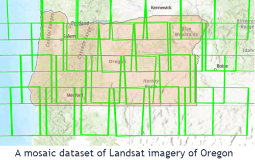
- Search for images within the extent of the Oregon state boundary, within a time range from 5/15/2022 to 10/15/2022, with a cloud cover criterion of less than 30%.
- Create a mosaic dataset from the search result. Below is the created mosaic dataset containing 229 scenes.
Create a Cloud-Free Image Composite
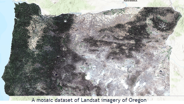
- Apply raster functions to remove clouds and shadows, perform pixel-based mosaicking, and clip using the study boundary.
- Create an image composite in a CRF format containing 7 surface reflectance bands.
Next, we’ll prepare additional indices as independent variables to work around image quality or spectral saturation in dense forest. I created band indices using the Band Arithmetic raster function:
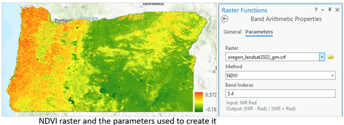
Leverage built-in options for NDVI, EVI, MNDWI, and SAVI: Below is the NDVI raster (left) and the parameters used to create it (right).
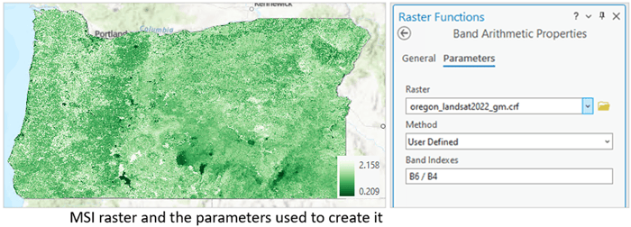
Use the user-defined option for MSI, RVI, and DIV: MSI (SWIR1/NIR) represents moisture stress index, RVI = NIR/R representing ration vegetation index, and DIV = NIR-R, representing difference vegetation index. An example of calculated MSI raster and the parameter used is illustrated below:
From this process, we have 7 Landsat surface reflectance bands, and 7 indices (NDVI, EVI, MNDWI, SAVI, MSI, RVI, and DVI) ready for subsequent use in training a regression model.
Process DEM Data
Following a similar workflow as the Landsat processing, all DEM data within same extent were selected, a DEM mosaic dataset was created from the search result, and a DEM of Oregon was clipped using the Clip Raster tool.
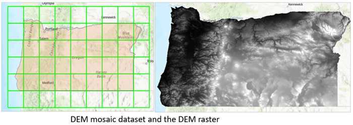
Additionally, a slope raster and an aspect raster were created using corresponding raster functions

The DEM, slope, and aspect will provide additional independent variables for training regression model.
Process GEDI Data
The GEDI data can also be accessed from Amazon Cloud. We can utilize the Earth Data portal to search data of our interest and save S3 paths of the search results. I created a trajectory dataset from the search result. This trajectory dataset is a file geodatabase dataset directly referencing the GEDI files in AWS. I then extracted the point data containing the aboveground biomass (AGBH field) within the study boundary. For the detailed steps on how to ingest GEDI data into ArcGIS, refer to this blog. below are the visuals of the created trajectory dataset and the exported point feature class with AGBH variable.
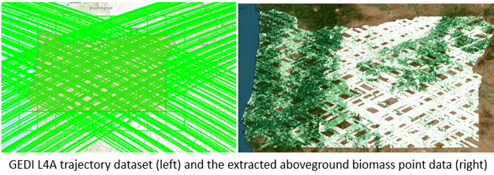
This point feature class will be used as the target in training regression model.
Train a Regression Model
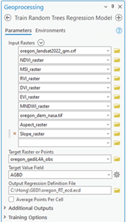
With all the input data prepared from the previous sections, we are now ready to train the model. Using the Train Random Tree Regression tool in the Image Analyst toolbox, I created a training model stored in .ecd file. This was achieved by using the extracted aboveground biomass point data as the training target, with the 7 band Landsat composite, derived indices, DEM, and calculated aspect and slope serving as independent variables.
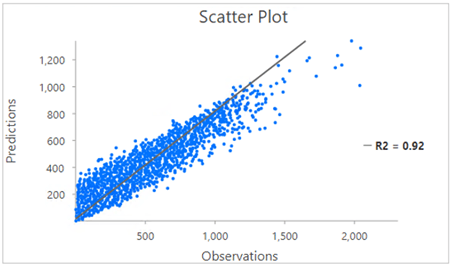
The scatter plot, with an R square of 0.92 when comparing observations and predictions, shows evidence of the model’s robust performance.
Create an Aboveground Biomass Raster
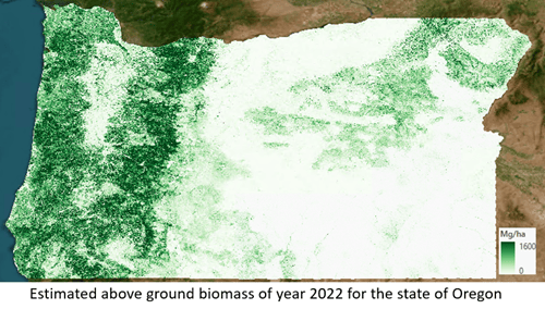
Moving to the next step, I used the Predict Using Regression Model tool, setting the input raster with the same set of rasters and in the same input sequence used during model training, along with the trained .ecd file. This process generated an above-ground biomass raster, an estimation for the entire state of Oregon, as shown below:
Conclusion
While the GEDI mission provides measurements for various variables like canopy height, leaf area index, and more, the synergy of different satellite data, optical and radar, can be harnessed to model these variables collectively. Leveraging ArcGIS Pro (3.2 and above) and remote-sensed datasets in the cloud enhances our ability to predict and understand these variables. I hope that this end-to-end biomass estimation workflow serves as an example and inspires you to explore other regions or variables across the planet.


Article Discussion: