

What is a materialized view?
Cloudera SQL Stream Builder (SSB) gives the power of a unified stream processing engine to non-technical users so they can integrate, aggregate, query, and analyze both streaming and batch data sources in a single SQL interface. This allows business users to define events of interest for which they need to continuously monitor and respond quickly.
There are many ways to distribute the results of SSB’s continuous queries to embed actionable insights into business processes. In this blog we will cover materialized views—a special type of sink that makes the output available via REST API.
In SSB we can use SQL to query stream or batch data, perform some sort of aggregation or data manipulation, then output the result into a sink. A sink could be another data stream or we could use a special type of data sink we call a materialized view (MV). An MV is a special type of sink that allows us to output data from our query into a tabular format persisted in a PostgreSQL database. We can also query this data later, optionally with filters using SSBs REST API.
Why use a materialized view?
If we want to easily use the results of our SQL job from an external application, MVs are the best and easiest way to do so. All we need to do is define the MV on the UI interface and applications will be able to retrieve data via REST API.
Imagine, for instance, that we have a real-time Kafka stream containing plane data and we are working on an application that needs to download all planes in a certain area, above some altitude at any given time via REST. This is not a simple task to do, since planes are constantly moving and changing their altitudes, and we need to read this data from an unbounded stream. If we add a materialized view to our SSB job, that will create a REST endpoint from which we will be able to retrieve the latest result from our job. We can also add filters to this request, so for example, our application can use the MV to show all the planes that are flying higher than some user-specified altitude.
Creating a materialized view
Creating a new job
An MV always belongs to a single job, so to create an MV we must first create a job in SSB. To create a job we will also need to create a project first which will provide us a Software Development Lifecycle (SDLC) for our applications and allows us to collect all our job and table definitions or data sources in a central place.
Getting the data
As an example we will use the same Automatic Dependent Surveillance Broadcast (ADS-B) data we used in other posts and examples. For reference, ADS-B data is generated and broadcast by planes while flying. The data consists of a plane ID, altitude, latitude and longitude, speed, etc.
To better illustrate how MVs work, let’s execute a simple SQL query to retrieve all of the data from our stream.
SELECT * FROM airplanes;
The creation of the “airplanes” table has been omitted, but suffice it to say airplanes is a virtual table we have created, which is fed by a stream of ADS-B data flowing through a Kafka topic. Please check our documentation to see how that’s done. The query above will generate output like the following:
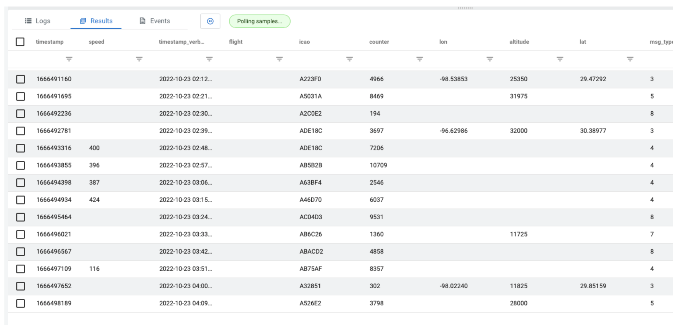 As you can see from the output, there are all kinds of interesting data points. In our example let’s focus on altitude.
Flying high
From the SSB Console, click on the “Materialized View” button on the top right:
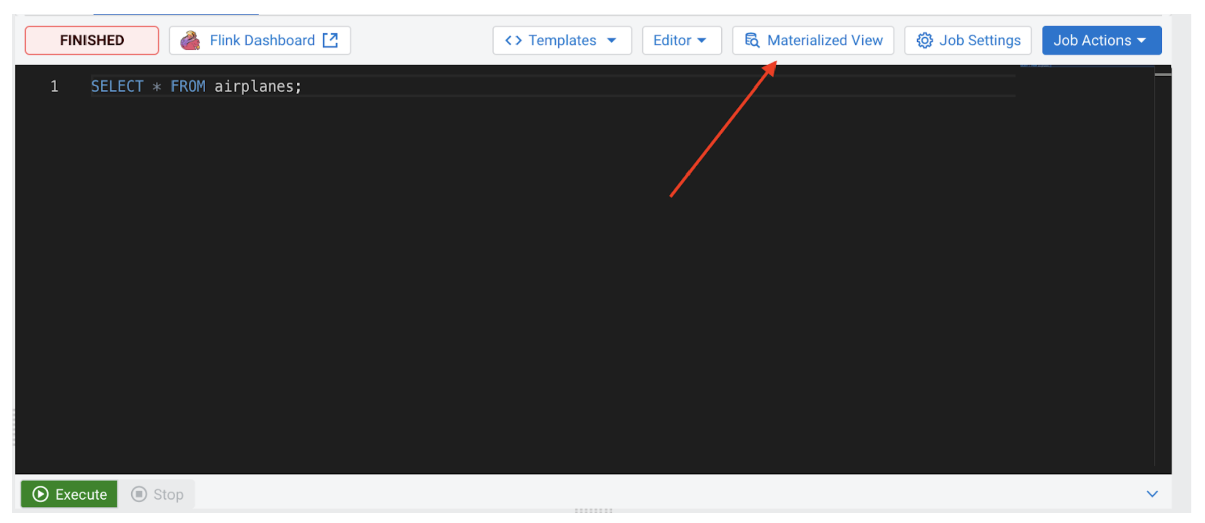
An MV configuration panel will open that will look similar to the following:
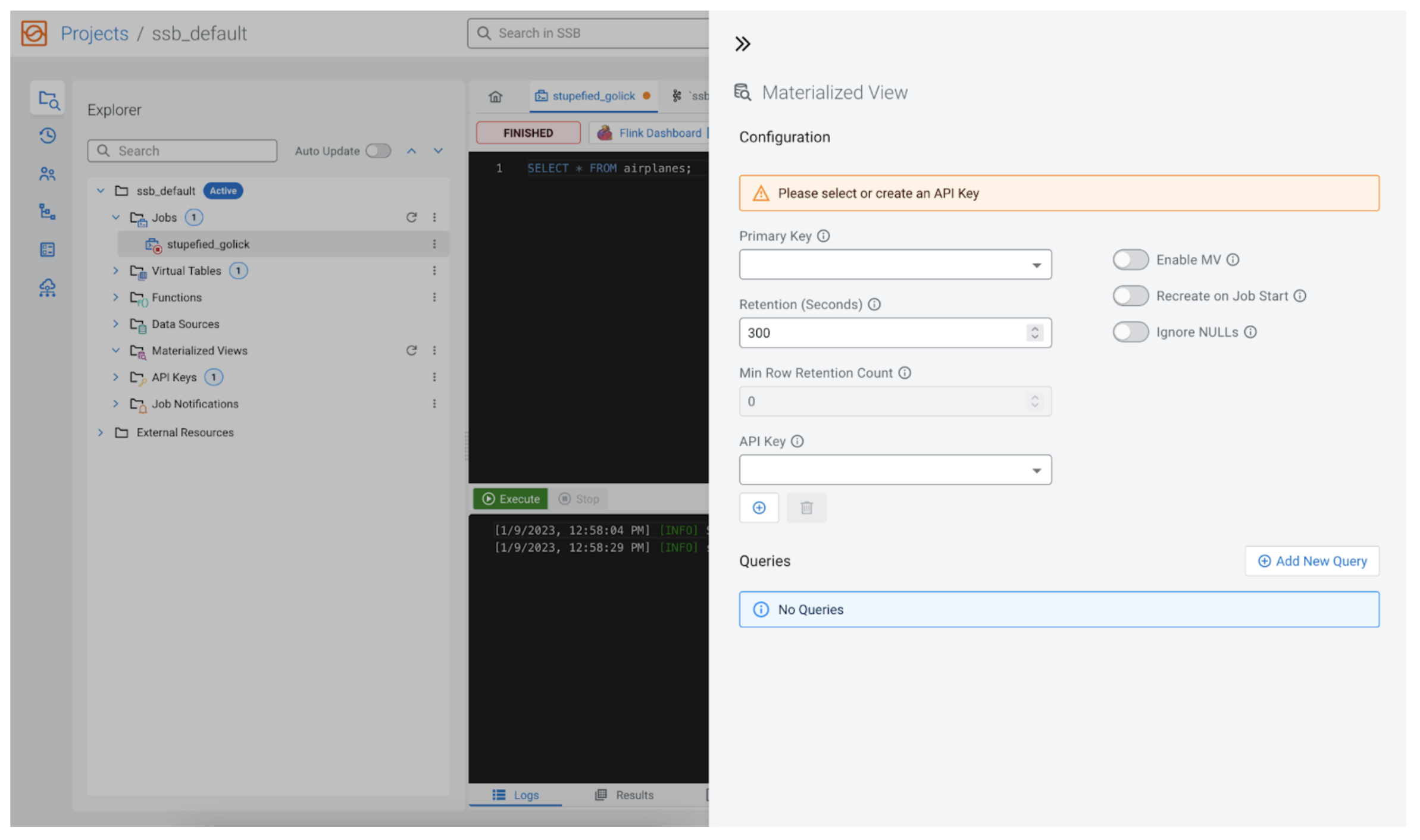
Configuration
SSB allows us to configure the new MV extensively, so we will go through them here.
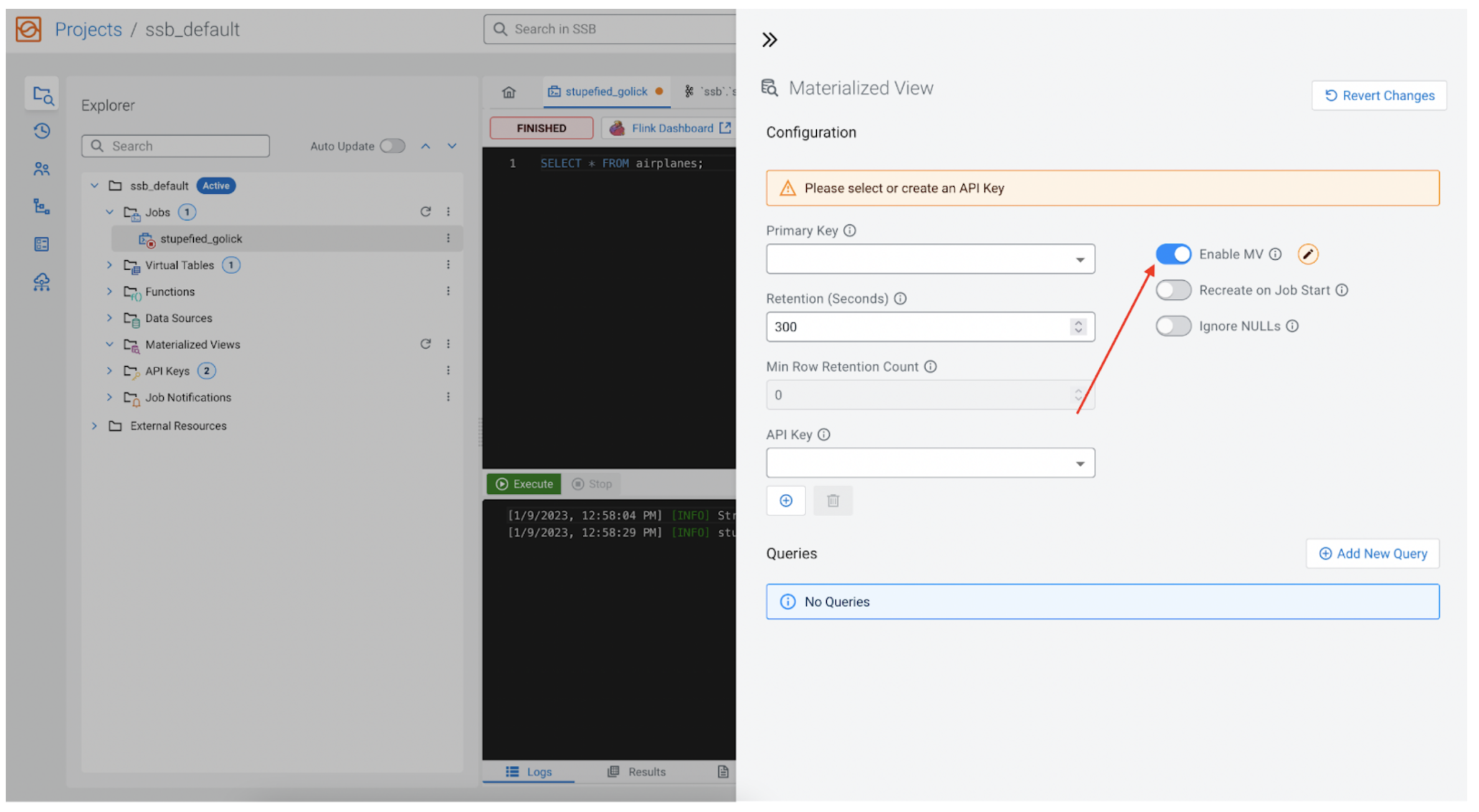
Enable MV
For the MV to be available once we have finished configuring it, “Enable MV” must be enabled. This configuration also allows us to easily disable this feature in the future without removing all the other settings.
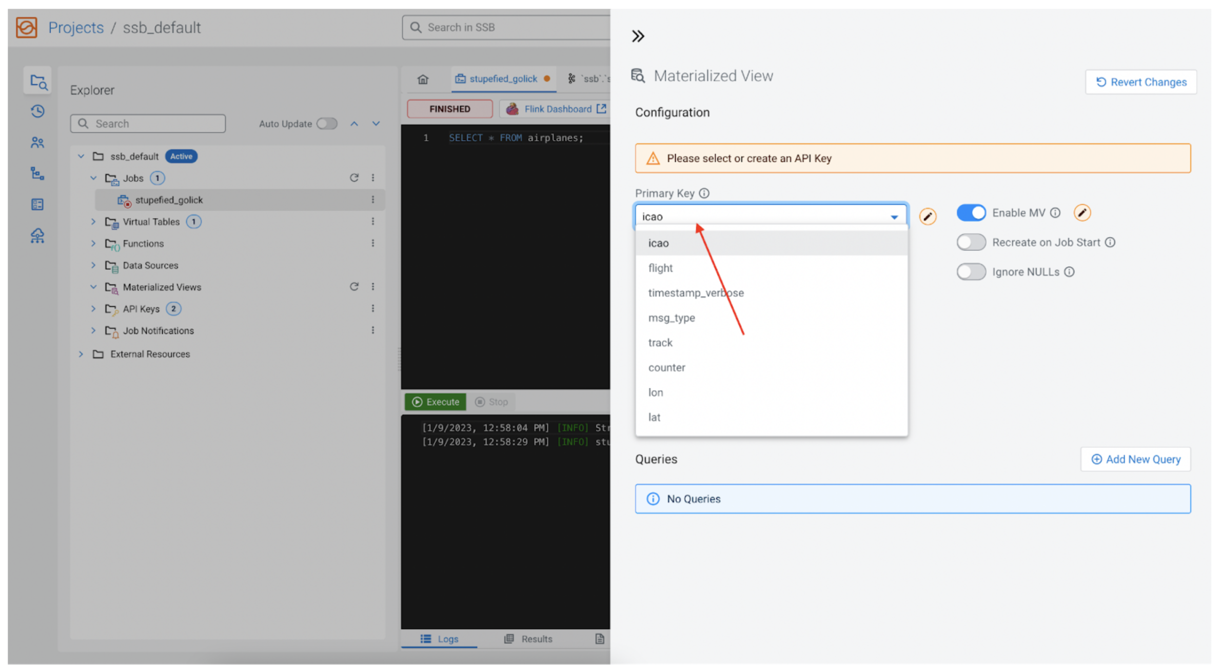
Primary key
Every MV requires a primary key, as this will be our primary key in the underlying relational database as well. The key is one of the fields returned by the SSB SQL query, and it is available from the dropdown. In our case we will choose icao, because we know that icao is the identification number for each plane, so it is a perfect fit for the primary key.
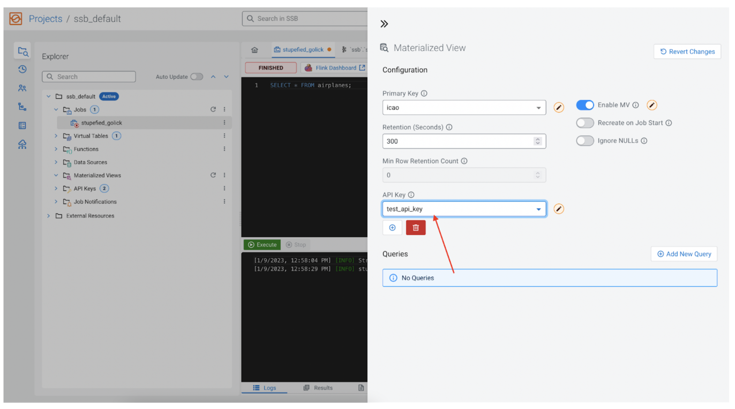
Retention and min row retention count
This value tells SSB how long it should keep the data around before removing it from the MV database. It is set to five minutes by default. Each row in the MV is tagged with an insertion time, so if the row has been around longer than the “Retention (Seconds)” time then the row is removed. Note, there is also an alternative method for managing retention, and that is the field below the retention time, called “Min Row Retention Count,” which is used to indicate the minimum number of rows we would like to keep in the MV, regardless of how old the data might be. For example we could say, “We want to keep the last 1,000 rows no matter how old that data is.” In that case we would set “Retention (Seconds)” to 0, and set “Min Row Retention Count” to 1,000.
For this example we will not change the default values.
API key
As mentioned earlier, every MV is associated with a REST API. The REST API endpoint must be protected by an API Key. If none has been added yet, one can be created here as well.
Queries
Finally we get to the most interesting part, selecting how to query our data in the MV database.
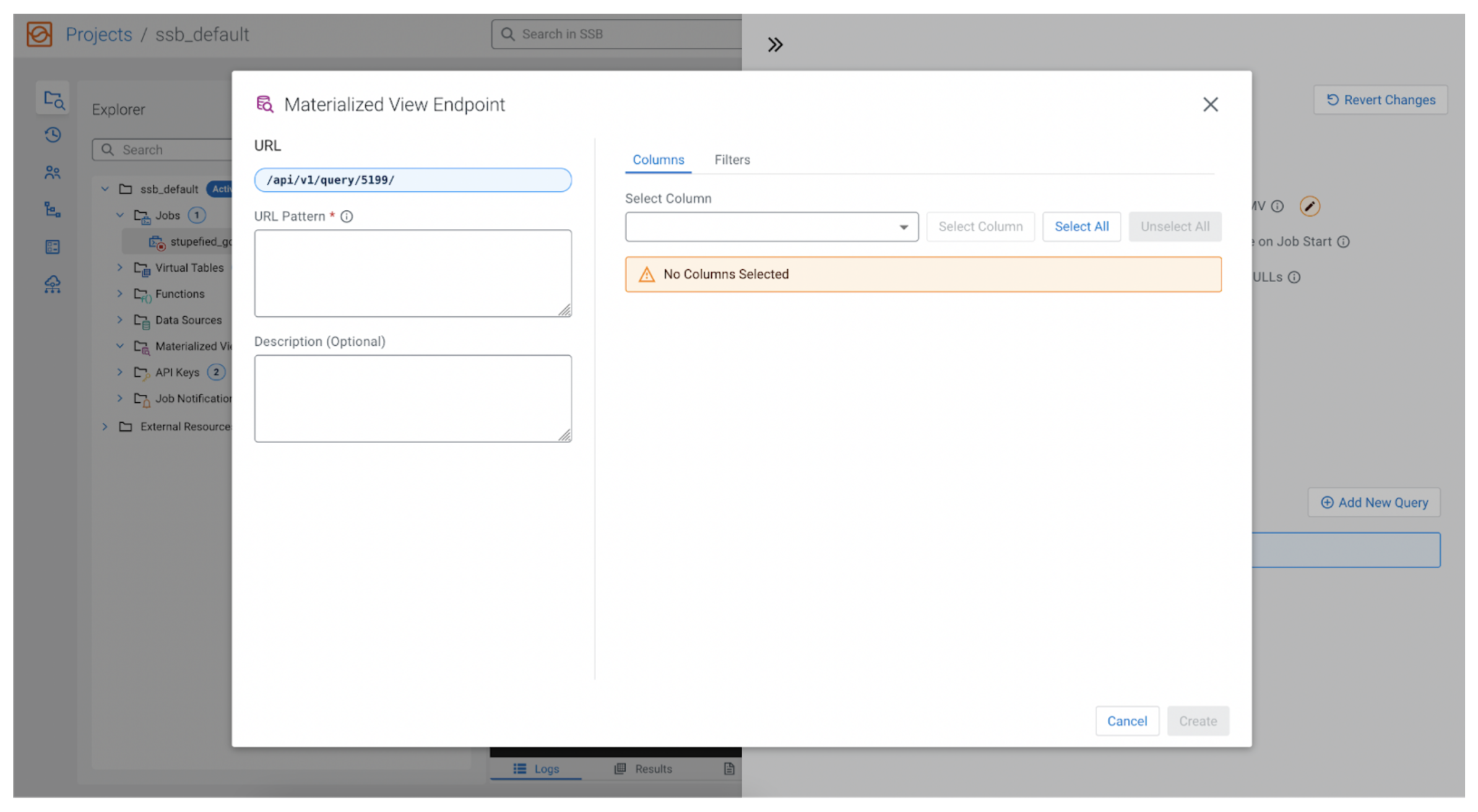
API endpoint
Clicking on the “Add New Query” button opens a pop-up that allows us to configure the REST API endpoint, as well as selecting the data we would like to query.
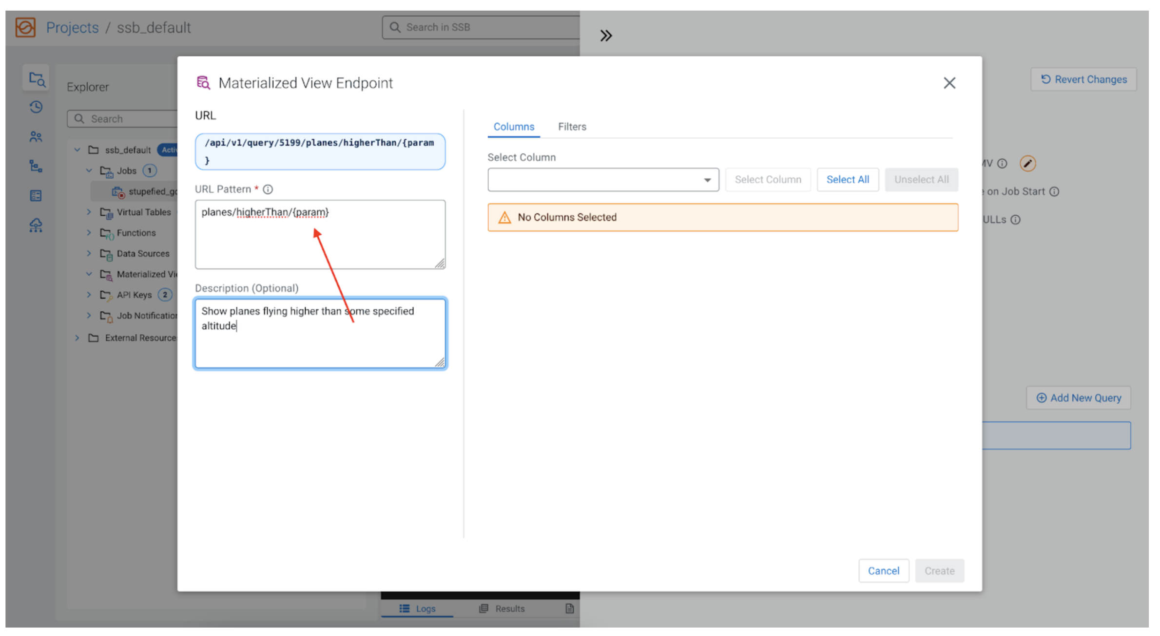
As we said earlier, we are interested in the plane’s altitude, but let’s also add the ability to filter the field altitude when calling the REST API. Our MV will be able to only show planes that are flying higher than some user specified altitude (i.e., show planes flying higher than 10,000 feet). In that case in the “URL Pattern” box we could enter:
planes/higherThan/{param}
Note the {param} value. The URL pattern can take parameters that are specified inside curly brackets. When we retrieve data for the MV, the REST API will map these parameters in our filters, so the user calling the endpoint can set the value. See below.
Choose the data
Now it is time to select what data to collect as part of our MV. The data fields we can choose come from the initial SSB SQL query we wrote, so if we said SELECT * FROM airplanes; the “Select Columns” dropdown will have things like flight, icao, lat, counter, altitude, etc. For our example let’s choose icao, lat, lon and altitude.
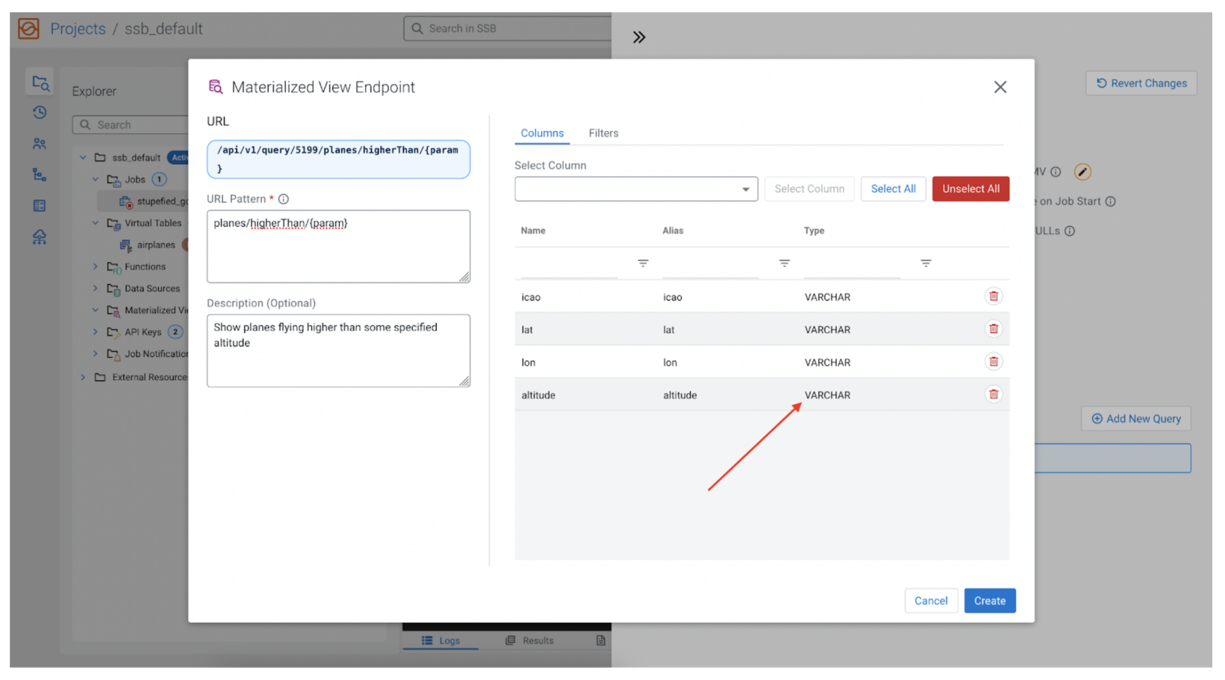
Oops
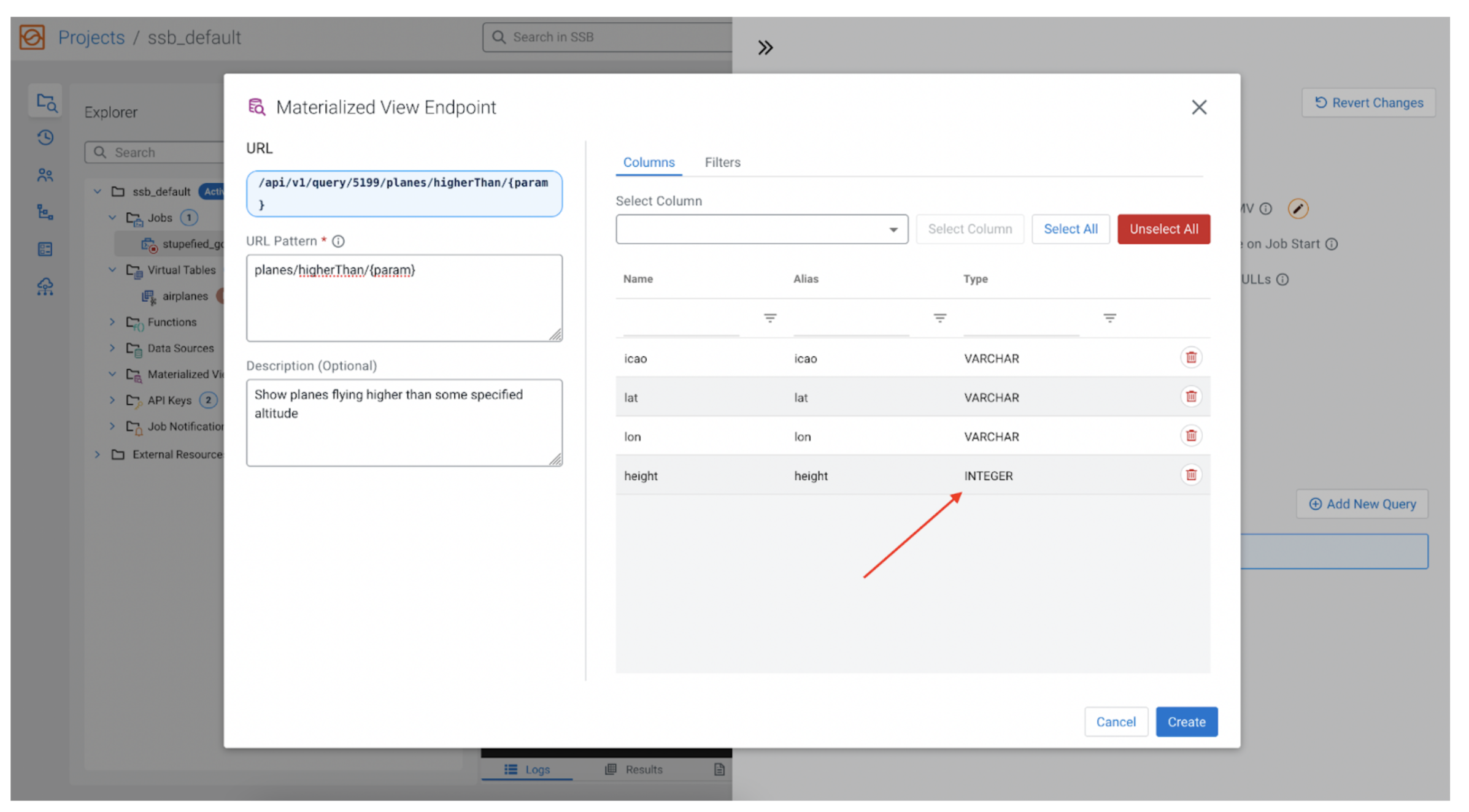
We have a problem. The data fields in the stream, including the altitude, are all of VARCHAR type, making it infeasible to filter for numeric data. We need to make a simple change to our SQL and convert the altitude into an INT, and call it height, to differentiate it from the original altitude field. Let’s change the SQL to the following:
SELECT *, CAST(altitude AS INT) AS height FROM airplanes;
Now we can replace altitude with height, and use that to filter.
Filtering
Now to filter by height we need to map the parameter we previously created ({param}) to the height field. By clicking on the “Filters” tab, and then the “+ Rule” button, we can add our filter.
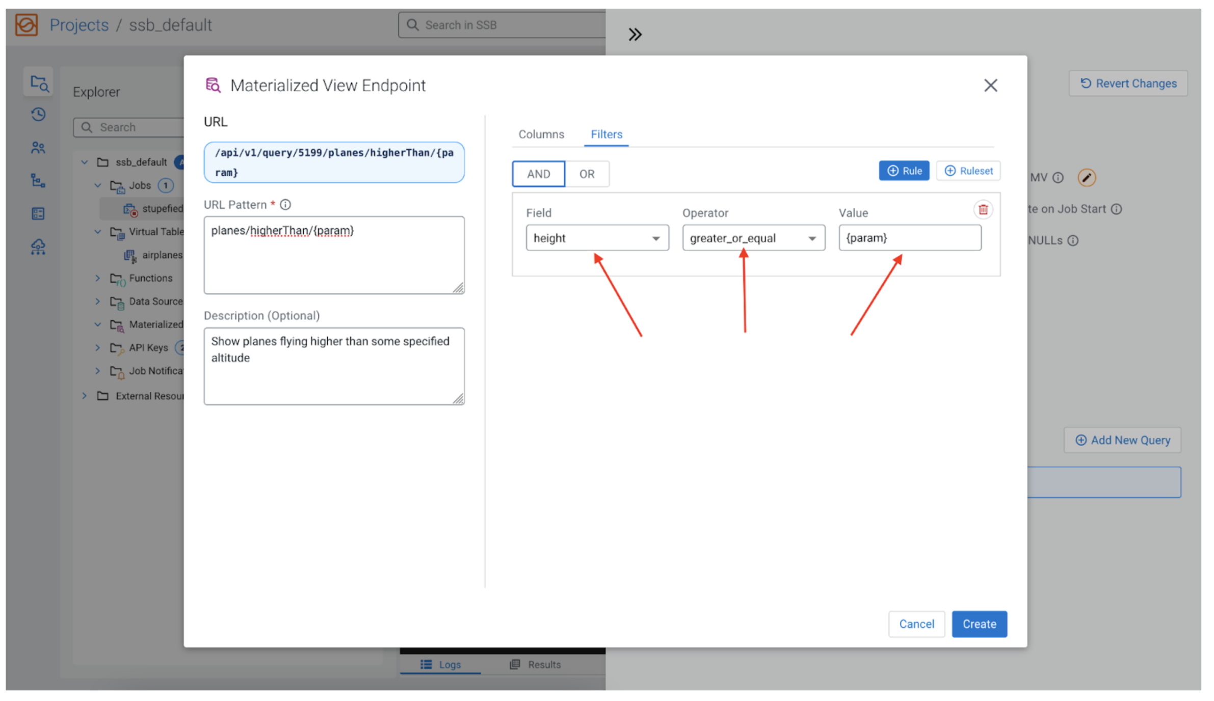
For the “Field” we choose height, for the “Operator” we want “greater_or_equal,” and for the “Value” we use the {param} we used in the REST API endpoint. Now the MV query will filter the rows by the value of height being greater than the value that the user would give to {param} when issuing the REST request, for example:
https://<host>/…/planes/higherThan/10000
That would output something similar to the following:
[{"icao":"A28947","lat":"","lon":"","height":"30075"}]
Conclusion
Materialized views are a very useful out-of-the-box data sink, which provide for the collection of data in a tabular format, as well as a configurable REST API query layer on top of that that can be used by third party applications.
Try it out yourself!
Anybody can try out SSB using the Stream Processing Community Edition (CSP-CE). CE makes developing stream processors easy, as it can be done right from your desktop or any other development node. Analysts, data scientists, and developers can now evaluate new features, develop SQL-based stream processors locally using SQL Stream Builder powered by Flink, and develop Kafka Consumers/Producers and Kafka Connect Connectors, all locally before moving to production in CDP.
Editor's Choice